
Note
This manual is the task-oriented guide to the wxPython Seedless GUI. It explains what to click, what to enter, what the generated input means, and what to check after a run. The companion Seedless Technical Manual contains the scientific background, the full input syntax, and the deeper discussion of optimisation and pulse design. The two manuals are intended to be read together.
The Seedless graphical user interface (GUI) provides an interactive environment for designing, running, and analysing optimal-control calculations performed by the seedless optimisation engine. It allows users to construct optimisation problems, launch calculations, and inspect the results without manually editing Seedless input files. The GUI generates the same input files used by the command-line version of Seedless, allowing calculations to be transferred seamlessly between the graphical and command-line environments.
This manual explains how to use the GUI effectively and is intended to complement, rather than replace, the Seedless Technical Manual. The technical manual describes the optimisation algorithms, pulse-design methodology, and complete Seedless input language, while this manual focuses on carrying out those tasks through the graphical interface. Throughout this guide, references are made to the Technical Manual whenever a deeper understanding of the underlying theory or input syntax may be helpful.
The GUI has been designed to support the normal workflow of pulse optimisation. A typical Seedless session consists of the following stages:
The chapters in this manual follow this same progression. New users are encouraged to work through the complete HNCO example presented later in this manual before exploring the remaining GUI features. Experienced users may prefer to use individual chapters as a reference for particular tasks or interface components.
Relationship to the Technical Manual
This manual explains how to perform pulse optimisation using the graphical interface. The theoretical background, optimisation methodology, and complete description of the Seedless input language are presented in the Seedless Technical Manual. Together, the two manuals provide a complete guide to using Seedless.
The Seedless GUI provides a graphical interface to the seedless pulse-optimisation engine. Rather than requiring users to edit Seedless input files manually, the GUI presents the most commonly used optimisation parameters through a structured interface. It assists in defining optimisation problems, configuring calculations, launching optimisations, and examining the resulting pulse sequences.
The GUI does not implement a separate optimisation engine. Every calculation is performed by the standard seedless program, using the same input files and producing the same output files as the command-line version. This ensures that calculations created with the GUI remain fully compatible with command-line workflows and can be exchanged freely between the two environments.
The GUI is intended to simplify routine tasks while preserving access to the full capabilities of Seedless. New users can construct optimisation problems using the guided workflow provided by the Wizard, whereas experienced users may prefer to work directly with the individual tabs or edit the generated input files manually.
In addition to preparing optimisation jobs, the GUI provides facilities for
Because the GUI uses the standard Seedless input and output formats, it is straightforward to move between graphical and command-line workflows. Users may therefore begin constructing an optimisation problem in the GUI and later refine the calculation by editing the input files directly if required.
See also
The optimisation methods, input keywords, and calculation strategies used by the GUI are described in detail in the Seedless Technical Manual. The GUI should be regarded as an alternative interface to the same optimisation engine rather than as a separate program.
Practical tip
For most applications, we recommend designing constant-amplitude, phase-only pulses using the highest practical B1 field permitted by your hardware. These optimisations are generally the fastest and most robust, and they often produce the best-performing pulses. Keep the pulse duration within the limits specified for your probe and amplifier. If a longer pulse is required, reduce the RF power accordingly. As a useful rule of thumb, halving B1 typically requires approximately doubling the pulse duration to achieve a similar infidelity. Since RF power scales approximately as B12, this reduces the power requirement by about a factor of four.
Installation and platform-specific configuration are described in the Seedless Technical Manual and are not repeated here. Before working through the examples in this guide, verify that the required software has been installed correctly and that the Seedless programs can be executed from your system.
In particular, confirm that:
Some optional features require additional software:
If these optional programs are not available, Seedless can still perform optimisations, although some plotting and report-generation features will be unavailable.
This worked example is the recommended first calculation after installing Seedless. It verifies that the GUI, the optimisation engine, and the supporting software are all functioning correctly while introducing the normal optimisation workflow.
Although the Run pulse collections action in the Templates tab executes a larger suite of demonstration calculations, it is recommended that new users begin with this single, well-characterised HNCO example. The same calculation is used throughout the Seedless Technical Manual, allowing the GUI workflow and the underlying input files to be compared directly.
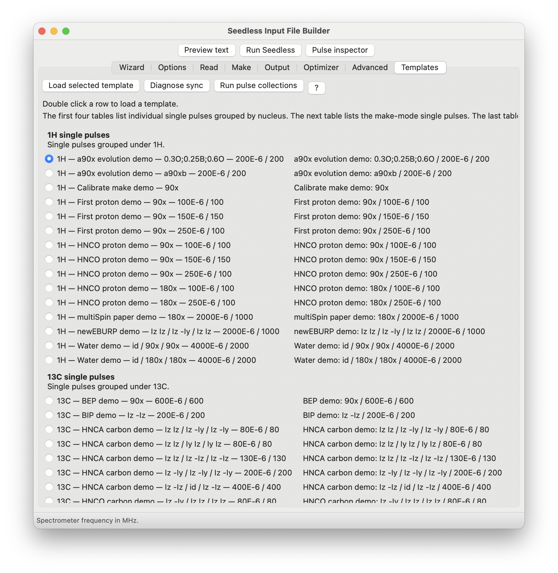
The GUI includes a collection of validated template calculations. Loading a template populates all of the required optimisation settings, providing a reliable starting point for learning the interface.
13 -HNCO HNCO demo - Iz -Iy / Iz Iz / Iz Iz - 80E-6 80
The Wizard provides a convenient overview of the optimisation problem. Confirm that the spectrometer, RF distribution, carrier frequency, plotting range, pulse duration, spin-system regions, and optimisation targets are all marked as configured. If desired, each setup dialog can be reopened to inspect or modify its settings.
The Calculation summary confirms that this example uses neither the Make nor the Read modes and that the optimisation is a constant-amplitude, phase-only pulse starting from random initial phases.
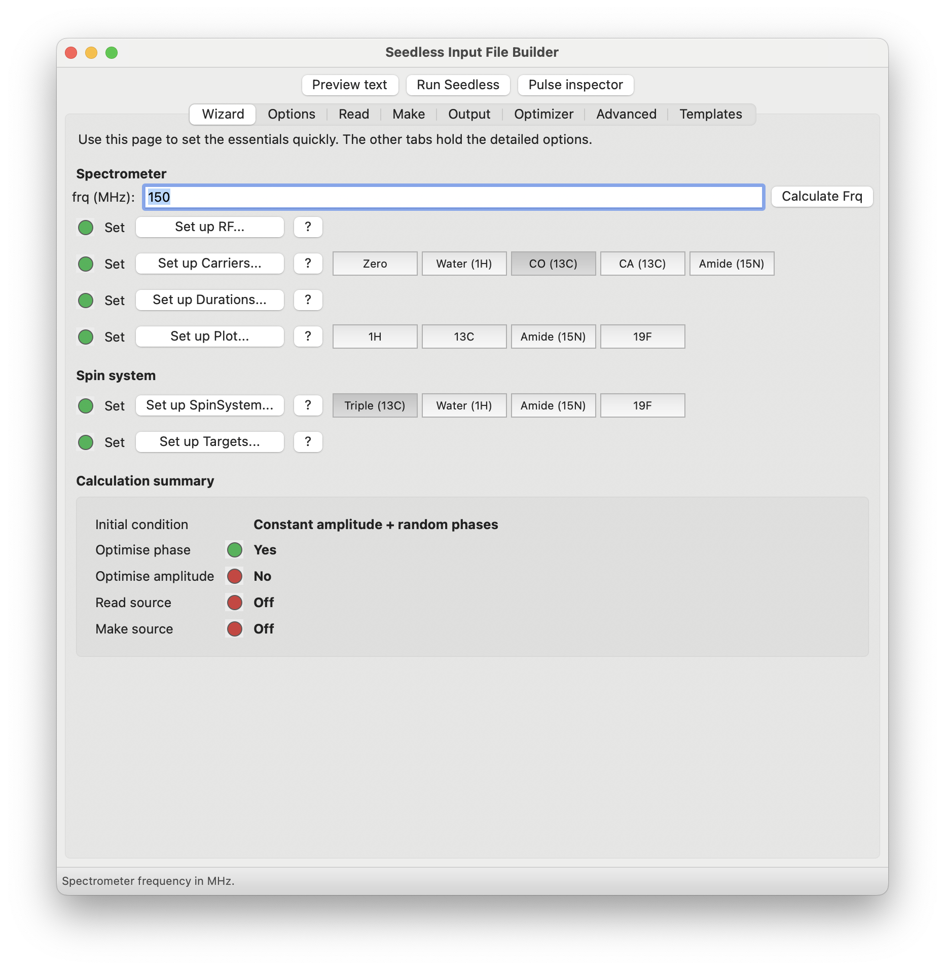
You can confirm that the spectrometer, RF distribution, carrier, plotting range, duration, spin-system regions, and targets are marked as set. You can open the setup dialog boxes to inspect the settings. The Calculation summary shows that we are not using the Make or Read modes, and that we are running a constant-amplitude phase-only pulse optimisation from random initial phases.
The Preview text window displays the Seedless input file that will be passed to the optimisation engine. This provides an important bridge between the graphical interface and the command-line version of Seedless: every option selected in the GUI is translated into the corresponding input keywords.
The principal scientific settings should correspond directly to the generated input. Reviewing this preview is one of the easiest ways to confirm that the optimisation problem has been specified correctly before launching a calculation.
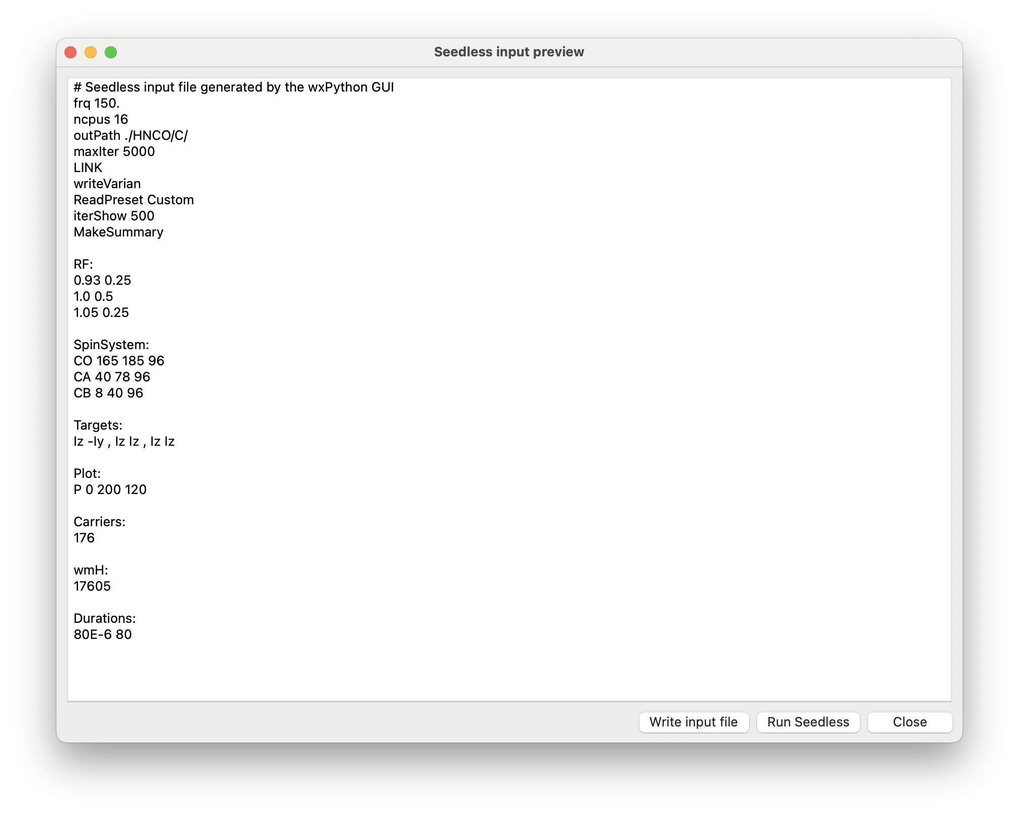
For the main scientific settings, you should see the same ideas represented in input syntax. This is the best place to check that the GUI settings have been translated correctly.
| GUI setting | Generated syntax | Meaning |
| Frq = 150 MHz | frq 150 | Larmor frequency of the optimised nucleus. |
| RF distribution | RF: rows | Relative B1 values and weights. |
| Carrier = 176 ppm | Carriers: then 176 | RF carrier position. |
| Maximum B1 = 17605 Hz | wmH: then 17605 | Maximum nutation frequency. |
| Duration = 80 μs, 80 points | Durations: then 80E-6 80 | Total duration and number of finite elements. |
| CO target Iz →−Iy | Iz -Iy | State-to-state excitation. |
The preview is the best place to detect an incorrect path, a missing RF-distribution row, an unintended optimisation target, or a unit conversion error before starting the optimisation. Correcting problems at this stage is usually much quicker than diagnosing them after a calculation has completed.
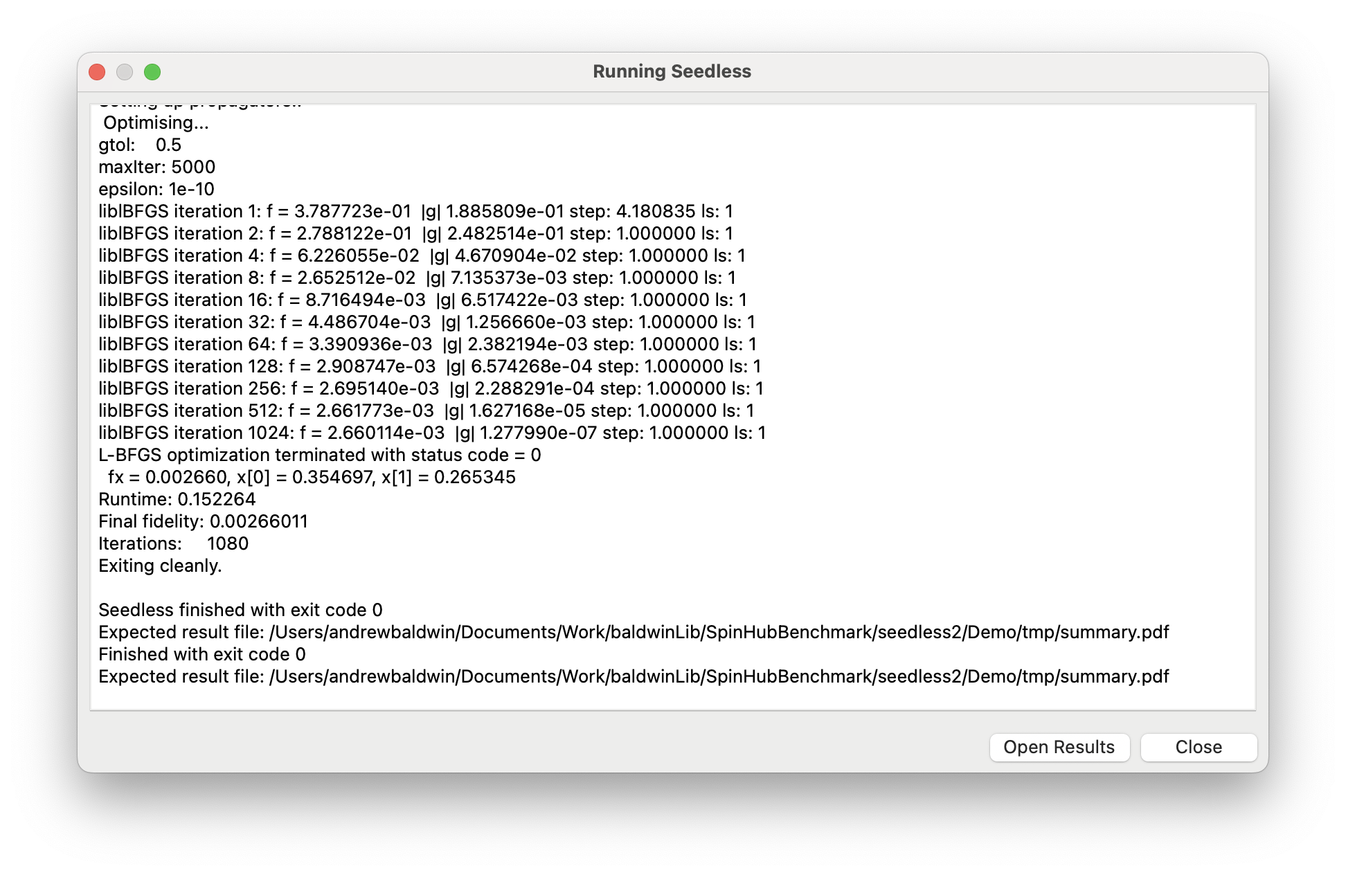
Click Run Seedless. A console dialog displays the program output. Wait for Exiting cleanly. The Open Results button then becomes available.
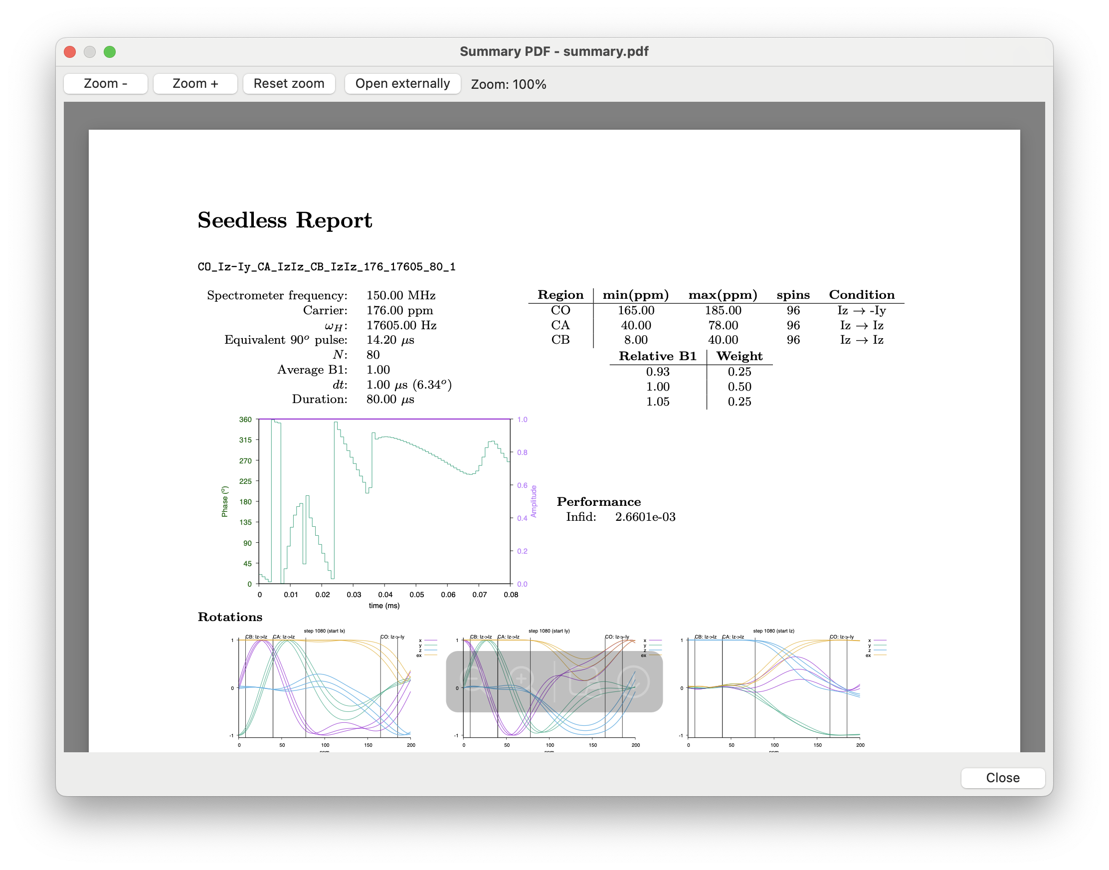
After the optimisation completes, open the summary report. Rather than simply confirming that the program finished, examine the results at four progressively more important levels:
Because the optimisation begins from random initial phases, the precise pulse shape and final infidelity will vary slightly between operating systems. Nevertheless, the overall pulse characteristics and the final infidelity should be comparable with the supplied example, typically around 2.7 × 10⁻³.
Note
This HNCO example is used throughout both the GUI Manual and the Seedless Technical Manual. Using a common reference calculation allows readers to move easily between the graphical workflow presented here and the more detailed discussions of optimisation strategy, input syntax, and report interpretation provided in the Technical Manual.
The Seedless GUI is organised around the normal workflow of pulse optimisation rather than around individual controls. Most users will progress through the interface in the following order:
The main window therefore places the three most frequently used actions at the top of the interface, with the notebook tabs providing access to progressively more detailed configuration options.
At the top of the window are three primary actions:
Displays the complete Seedless input file that will be generated from the current GUI settings. This is the quickest way to verify that the optimisation problem has been configured correctly before starting a calculation.
Writes the generated input file and launches the optimisation using the standard Seedless engine.
Searches recursively below the current working directory for pulse files and their associated reports, providing convenient access to both current and previous optimisation results.
After an optimisation has completed, the run dialog’s Open Results button opens the report generated by the current calculation. The top-level Pulse inspector (the built-in pulse browser) provides a separate browser for locating and reviewing both current and archived optimisation results.
The notebook contains eight tabs, each corresponding to a particular stage of the optimisation workflow:
Defines the physical optimisation problem, including the spectrometer, spin system, optimisation targets, and pulse design.
Controls project organisation, file locations, naming conventions, batch relationships, and selected advanced options.
Imports an existing pulse or configures an optimisation that begins from a previously generated pulse.
Constructs or calibrates built-in pulse shapes before optimisation.
Controls spectrometer conventions, pulse-file formatting, and exported output.
Specifies optimisation algorithms, convergence criteria, iteration limits, CPU usage, and related numerical settings.
Provides specialised options for analysis, diagnostics, propagation methods, evolution calculations, and data conversion.
Gives access to validated example calculations and collections of demonstration pulses that provide reliable starting points for new optimisation problems.
Question-mark buttons throughout the interface provide concise contextual help for individual controls. They are intended as quick reminders of each option’s purpose. More detailed discussions of optimisation methods, pulse-design strategy, and the corresponding Seedless input keywords are provided in the Seedless Technical Manual.
The Help menu provides access to the GUI Manual, the Seedless Technical Manual, and a selection of publications describing the pulse-design methods implemented by Seedless. The Seedless menu contains commands for loading a GUI session from an existing pulse, importing a Seedless input file into the GUI, opening the Pulse Inspector (the built-in pulse browser), and launching optimisation calculations.
A reliable strategy is to begin with the template that most closely matches your intended experiment, save it under a new filename, and then modify one group of settings at a time. This approach makes it much easier to identify the effect of each change and avoids introducing several independent sources of error simultaneously.
The Wizard defines the physical pulse-design problem: the spectrometer, RF field, chemical-shift regions, optimisation targets, and pulse duration. The remaining tabs mainly control how Seedless performs the optimisation and how the results are written or analysed.
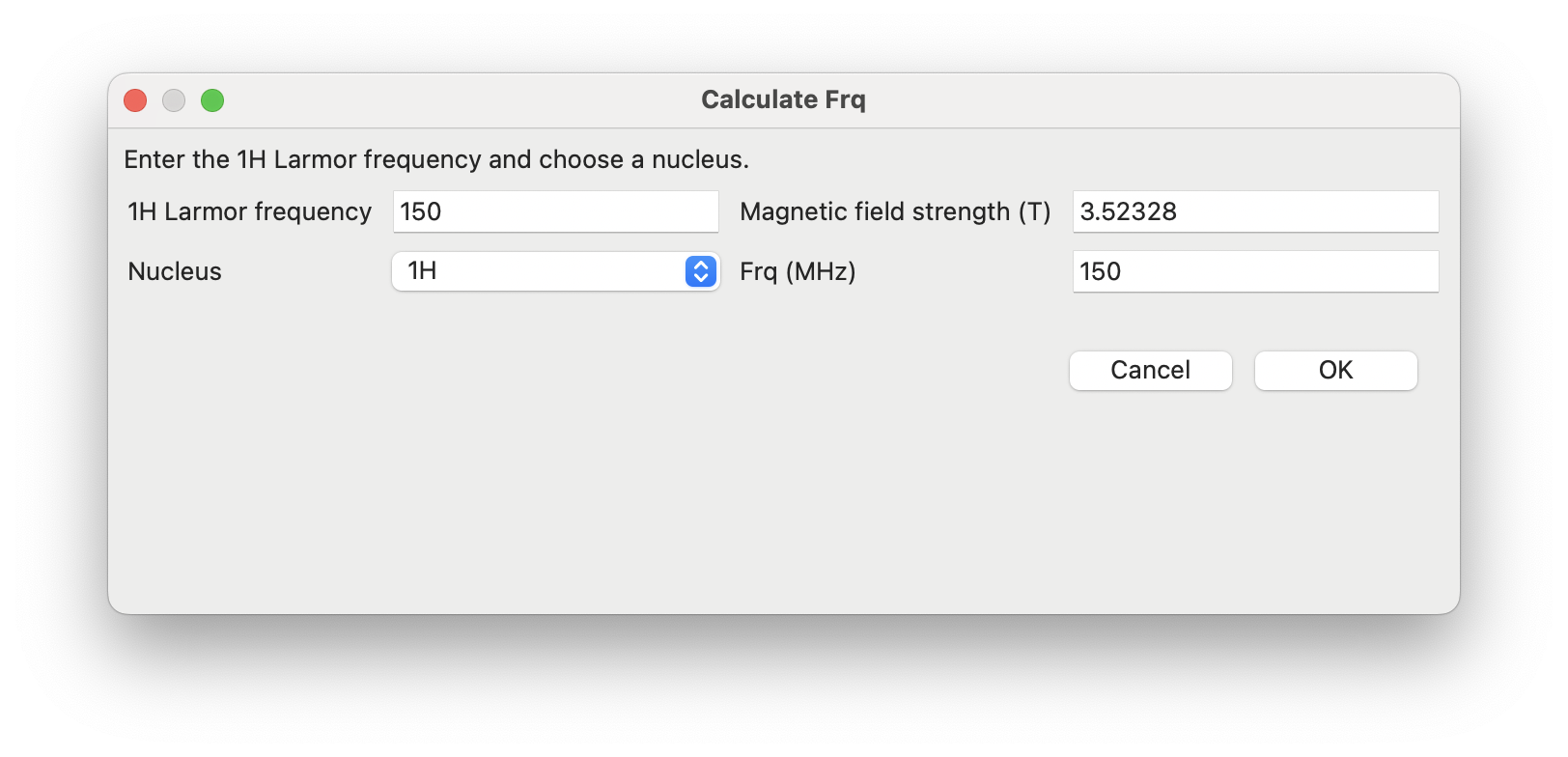
Begin by defining the spectrometer frequency for the nucleus of interest in MHz. Click Calculate Frq, enter either the proton frequency or the magnetic field strength, select the nucleus of interest, and allow the dialog to calculate the corresponding nucleus frequency automatically. Or specify the value you need directly. The generated header is frq value (Figure 6).
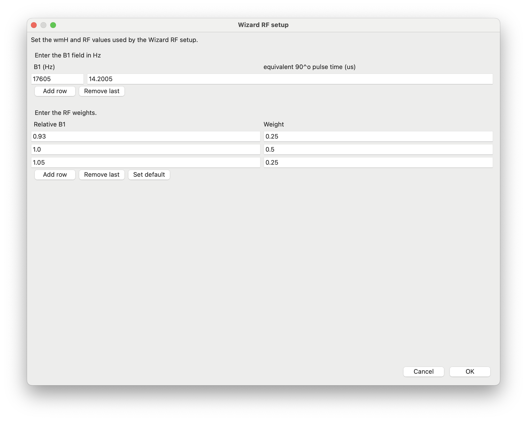
Click Set up RF (Figure 7). The upper table sets wmH, the central nutation frequency in Hz (ν1). Measure or obtain the relevant RF calibration for the actual probe and sample. Accurate RF calibration is essential because every subsequent optimisation assumes that the specified RF field represents the experimental hardware. Errors introduced here cannot usually be corrected later by the optimisation. A 90-degree pulse of duration t90 corresponds to

The lower table sets the relative B1 distribution and weights written under RF: to compensate for field inhomogeneity. A simple three-point distribution is a useful starting model, but it should be adapted when experimental calibration supports a different distribution.
Warning
Before using a new pulse experimentally, follow the probe and spectrometer manufacturer’s limits for RF field, pulse duration, duty cycle, and sample heating. Do not assume that a higher B1 is always safer or better. A good starting point is the highest practical B1 for your hardware; then determine the pulse duration needed to reach the desired performance, and reduce B1 only if necessary to stay within the hardware limits. As a rough rule of thumb, halving B1 often requires roughly doubling the pulse duration to achieve a similar infidelity, while the RF power requirement falls by about a factor of four.
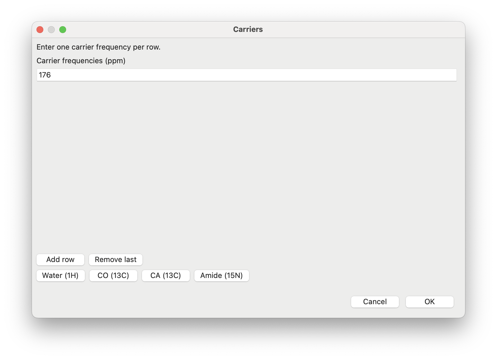
Click Set up Carriers (Figure 8). The carrier frequency defines the centre of the optimisation window. Enter one carrier position (in ppm) per row. Multiple rows request separate optimisations using identical pulse settings but different carrier frequencies. More than one row requests multiple calculations. The values are written under Carriers:.
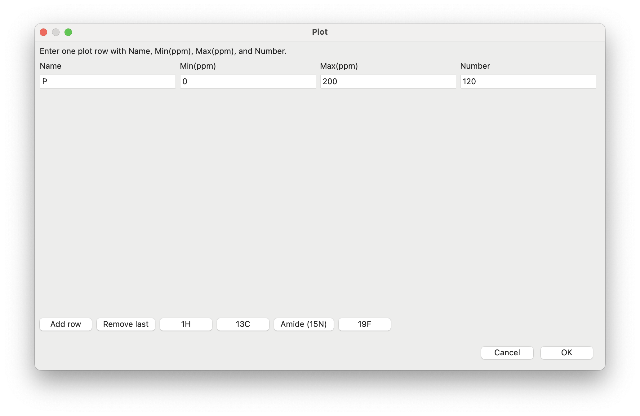
Click Set up Plot (Figure 9). Each row has a label, minimum ppm, maximum ppm, and number of validation points. The plotting grid is used only to evaluate the finished pulse; it does not influence the optimisation itself. By testing the pulse at many more frequencies than were used during optimisation, the plotting grid reveals whether the pulse interpolates smoothly across the desired bandwidth. As a starting point, use three or four times as many plotting points per ppm as optimisation points.
Practical tip
It is important that your pulse performs well not just at the specific chemical shifts used for the optimisation, but also between them. By setting more points in the plotting grid than in the optimisation grid, you can quickly check that the pulse performs well across the full band.
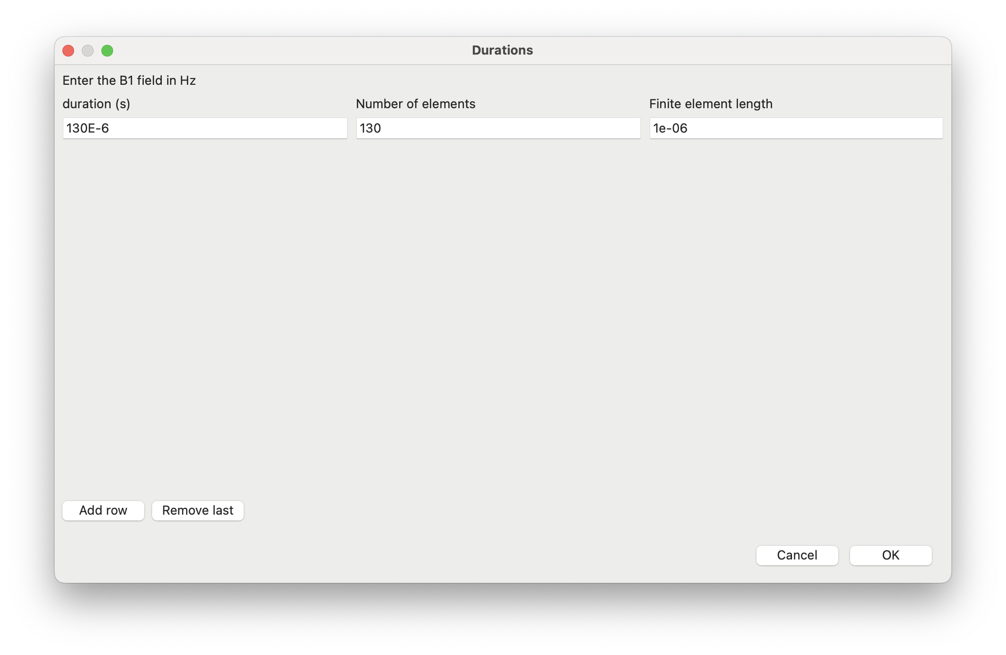
Click Set up Durations (Figure 10). Enter total duration in microseconds and the number of finite elements. The dialog shows the element length. Rows are written under Durations:; multiple rows request multiple calculations.
Finite elements of roughly 1–2 μs are a practical starting point for many liquid-state NMR applications, but hardware response and the required bandwidth may justify different values. The Technical Manual discusses the trade-off in more detail.
Shorter finite elements provide greater freedom for the optimisation, but they also increase the number of optimisation variables and may place greater demands on the spectrometer hardware (and increase the time needed for optimisation).
Practical tip
Finite elements can be very short on modern NMR hardware, but extremely short elements are more vulnerable to transient response. When the spectrometer changes phase or amplitude from one element to the next, there can be short transients before the hardware stabilises. For that reason, it is usually desirable to keep the finite element as long as practical. Once you have settings that work for your pulse, try to increase the finite-element length as much as you can while maintaining the desired performance.
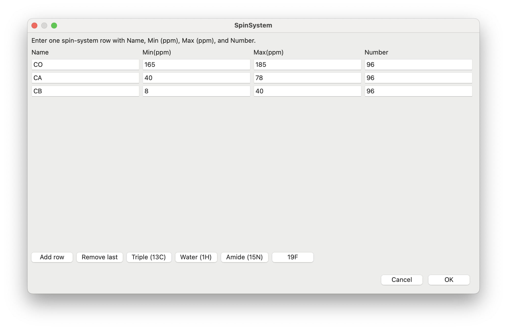
Click Set up SpinSystem (Figure 11). Each row defines one chemical-shift region over which the pulse should achieve the specified target. The optimisation samples the region using the requested number of points and attempts to satisfy the target throughout the entire band rather than only at its centre. Add one row for each chemical-shift band, giving a name, minimum ppm, maximum ppm, and number of optimisation samples. These rows are written under SpinSystem:.
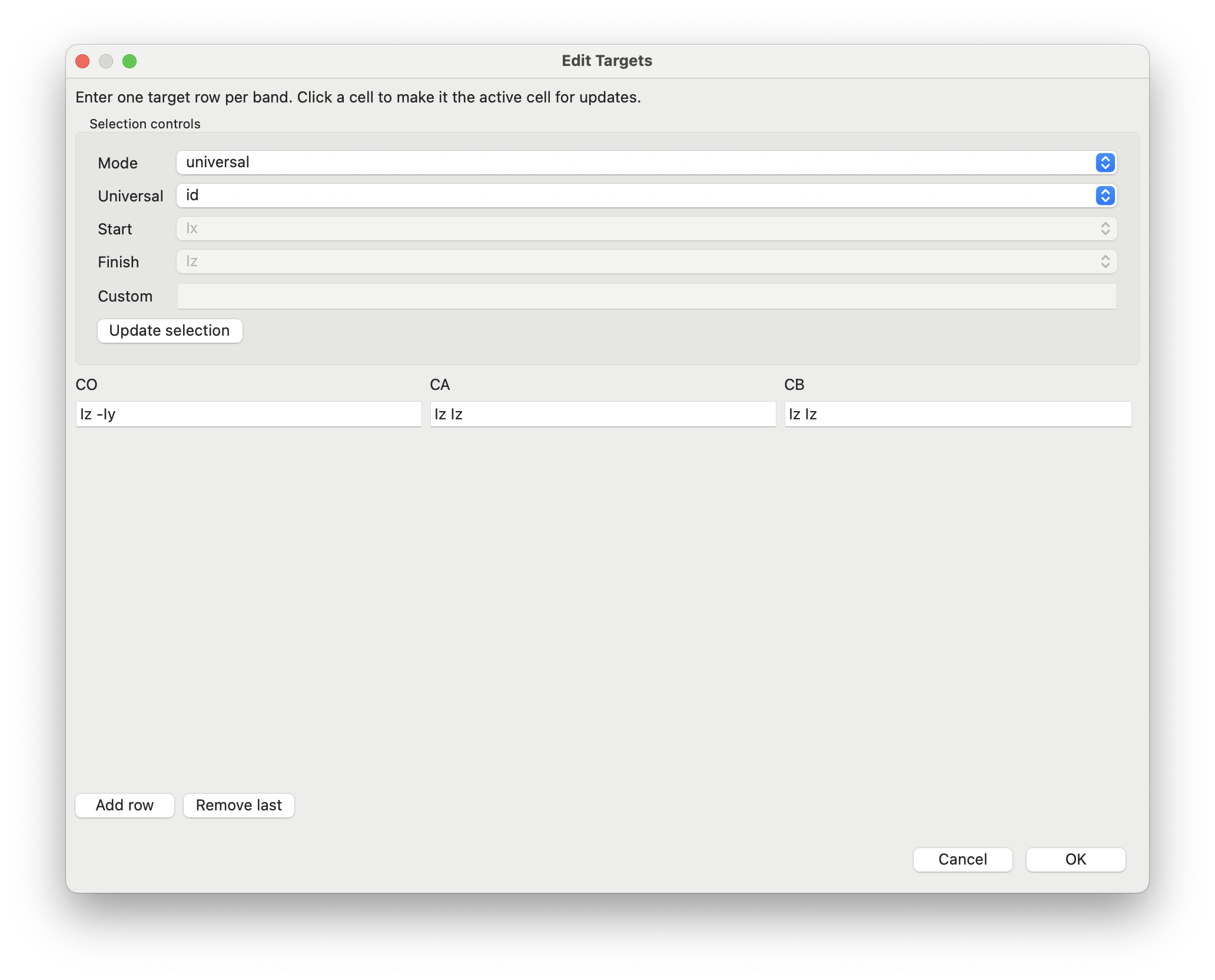
Click Set up Targets (Figure 12). The optimisation target specifies the transformation that Seedless should produce within each spin-system region. There must be one target cell for every spin-system band. The editor supports:
an operation such as 90x, 180x, or id that controls the full rotation.
a start and finish such as Iz -Iy; this controls only the transformation required by the experiment.
a target such as Iz Iex, placing magnetisation in the transverse plane without fixing its phase.
specialised syntax described in the Technical Manual.
Use a universal target when the pulse must replace an ideal rotation in several contexts. Use state-to-state when only one known starting state matters. Choosing the simplest target that satisfies the experimental requirements generally makes the optimisation easier and often produces shorter, lower-power pulses.
Checkpoint
At this point the physical pulse-design problem is completely specified. The virtual spectrometer, RF calibration, chemical-shift regions, optimisation targets, and experimental constraints have all been defined. The remaining notebook tabs control how Seedless searches for the pulse, how results are written to disk, and how existing pulses are analysed or converted. Most of the options will not be used in a typical workflow.
After an optimisation has completed, the next step is to determine whether the resulting pulse is suitable for the intended experiment. The Pulse Inspector provides a convenient way to browse all Seedless pulses beneath the current working directory together with their associated reports.
Select a row to preview a pulse. Use Open file to inspect the generated Seedless input or output files, and double-click a row to open the corresponding summary PDF. The Pulse Inspector can therefore be used both to examine the results of the current optimisation and to revisit previously generated pulse collections.
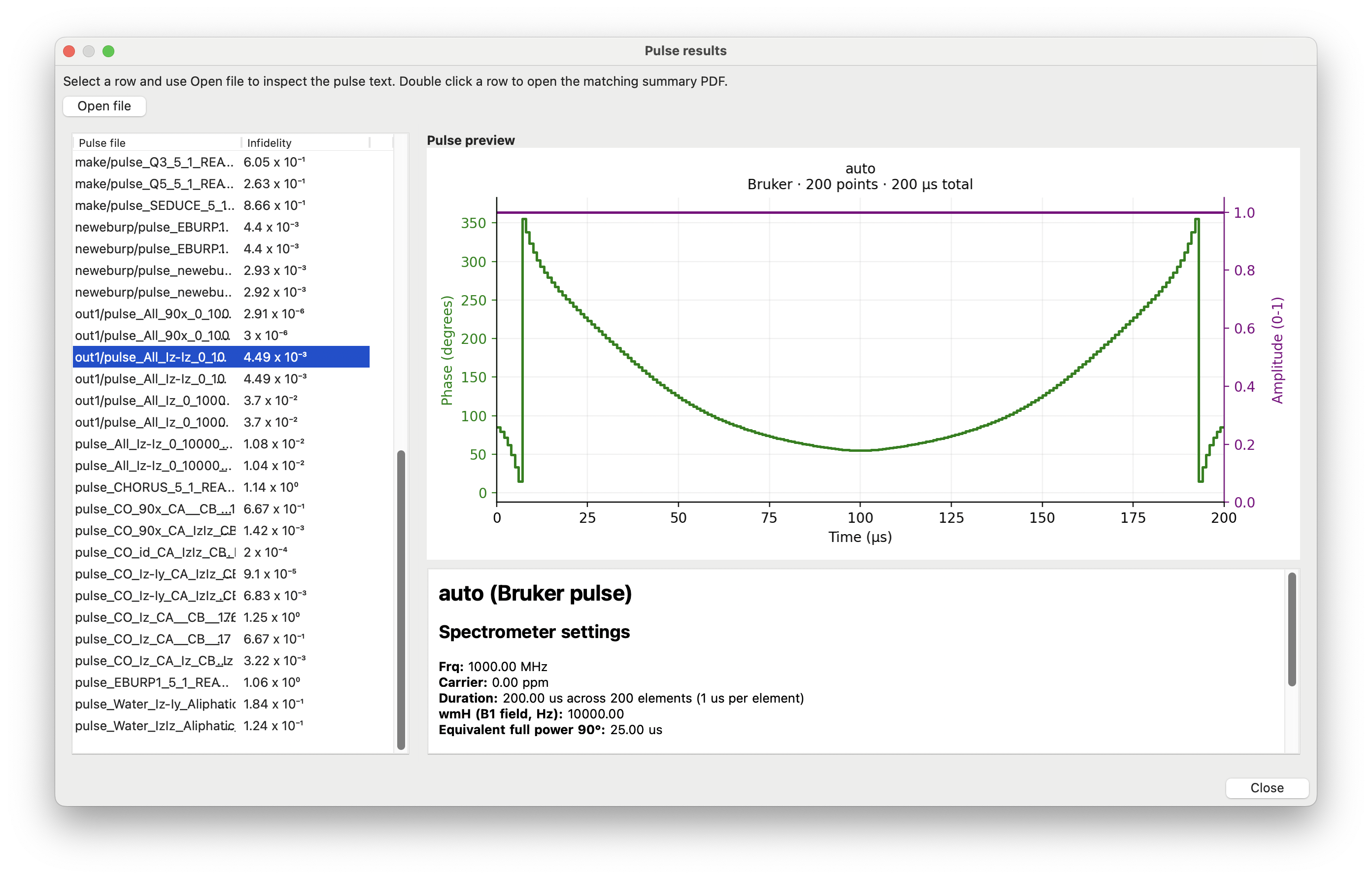
When reviewing the summary report, it is helpful to examine the results in a consistent order. Rather than concentrating solely on the final infidelity, consider the following questions.
The Seedless Technical Manual discusses the interpretation of optimisation reports, convergence behaviour, and performance plots in much greater detail. The purpose of the GUI Manual is to provide a practical framework for deciding whether a pulse is ready for experimental use or whether it should be refined further.
The Wizard is the recommended way to define a new pulse-design problem and will be sufficient for most routine optimisations. The remaining notebook tabs provide access to project management, specialised optimisation modes, pulse import and export, advanced analysis, and detailed control of the optimisation engine.
For a first optimisation, it is usually best to leave these settings at their template defaults unless you have a specific reason to change them. As you become more familiar with Seedless, the tabs provide progressively finer control over how optimisations are performed and how results are analysed.
This section describes the purpose of each tab, the settings that most users are likely to change, and the situations in which the more specialised options become useful.
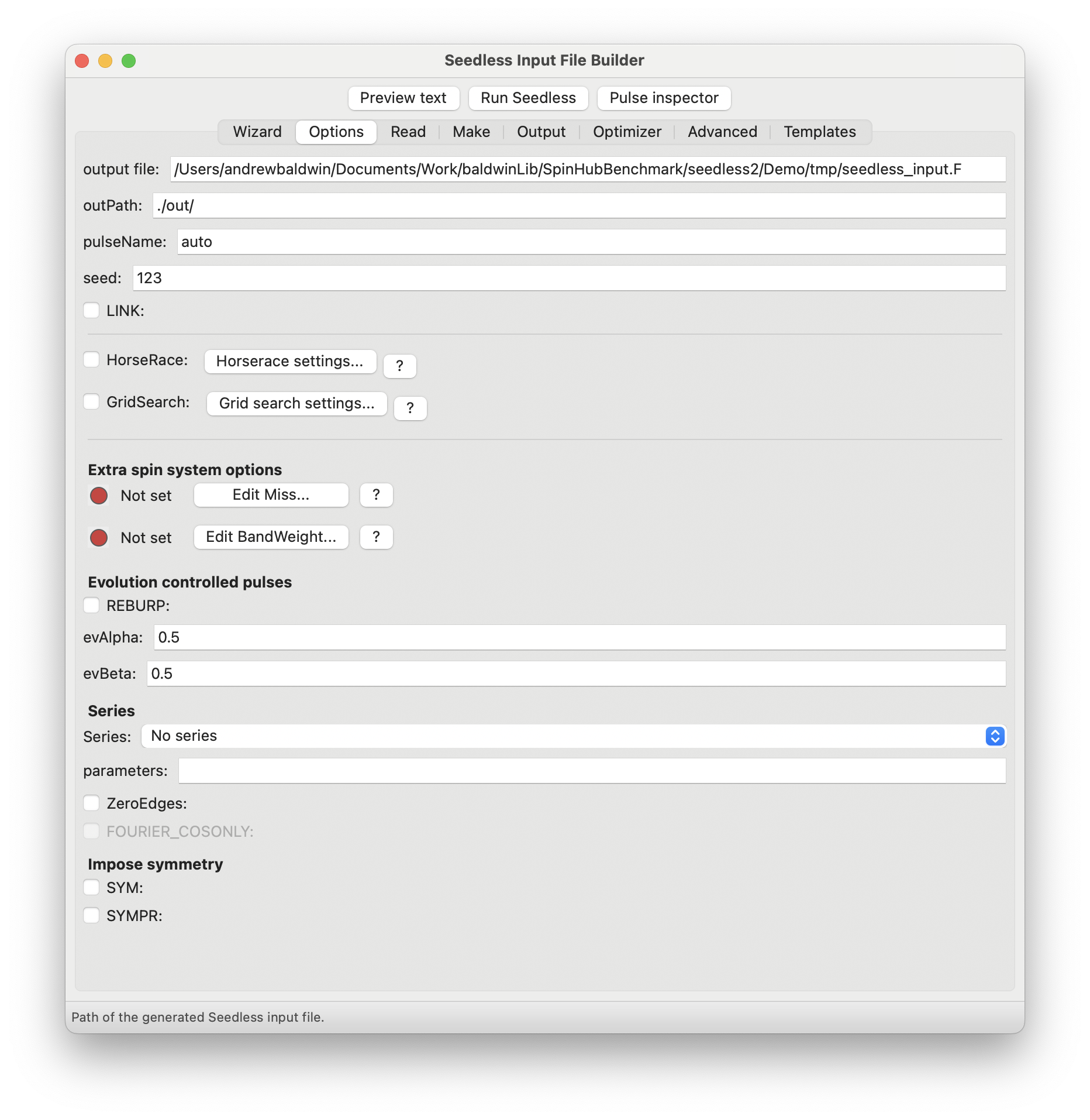
For routine work, check the following first:
where the generated input script is written. An existing file at this location may be overwritten.
Directory in which optimisation results, pulse files, and reports are written. Using a separate output directory for each project helps keep related calculations together.
User-defined name for generated pulses, or auto to create descriptive filenames automatically.
random-number seed, useful for reproducing a run.
pairs target rows and duration rows instead of forming every combination.
The remainder of the Options tab contains advanced optimisation modes. These are intended for situations where the default optimisation strategy is no longer sufficient. Most users will encounter them only after gaining experience with routine pulse optimisation or when following a supplied template.
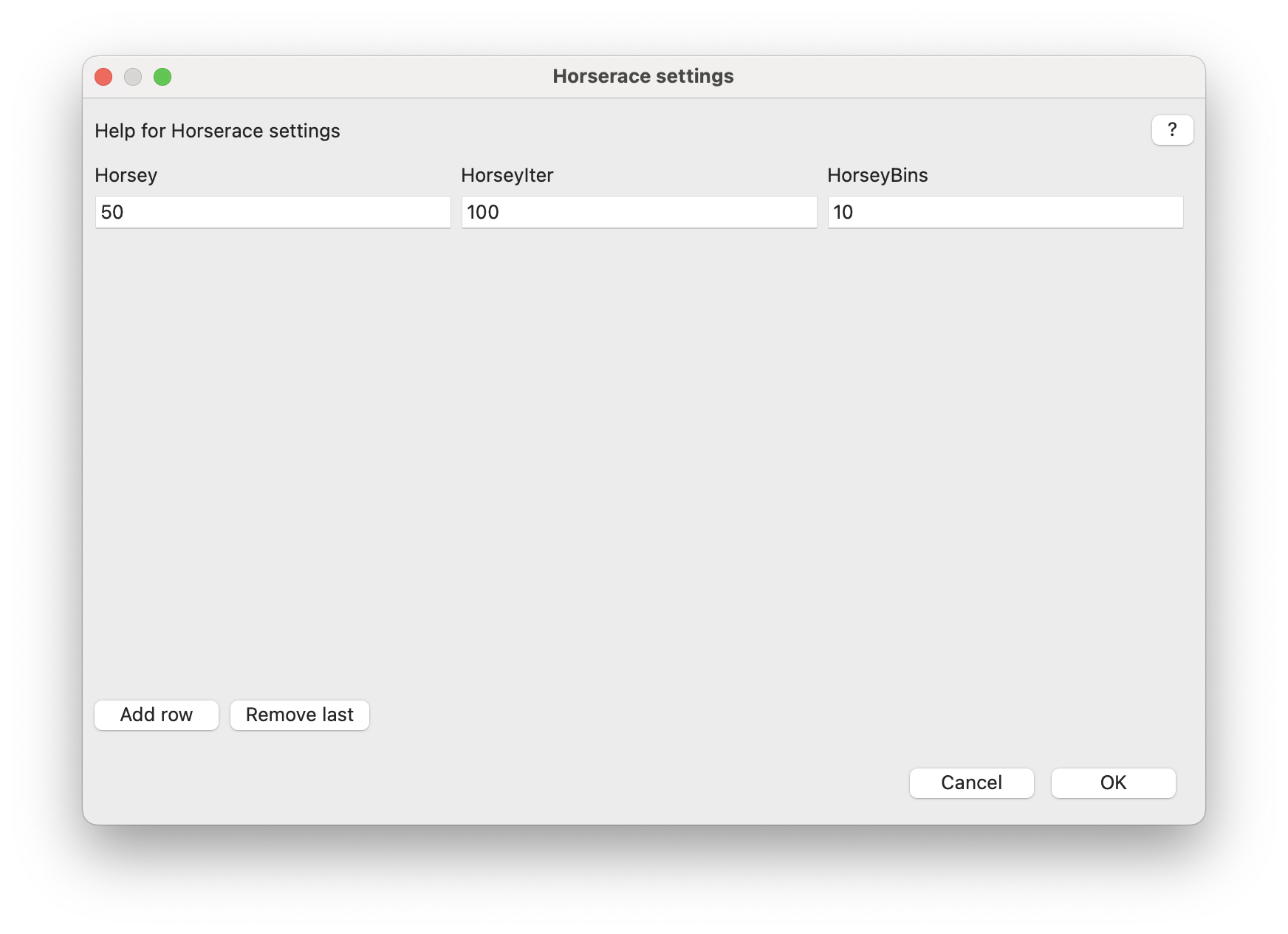
Repeats an optimisation using different random-number seeds (Figure 15). This is useful when optimisation performance varies significantly between runs, allowing the most successful result to be identified. Seed depednence is relatively rare. The Technical Manual explains this in more detail.
Performs a systematic exploration of pulse duration, maximum B1, finite-element length, or other selected parameters. Grid searches are often useful when selecting practical pulse-design constraints before beginning a full optimisation.
use when a restraint should also be applied during the pulse, not only at the end (Figure 16).
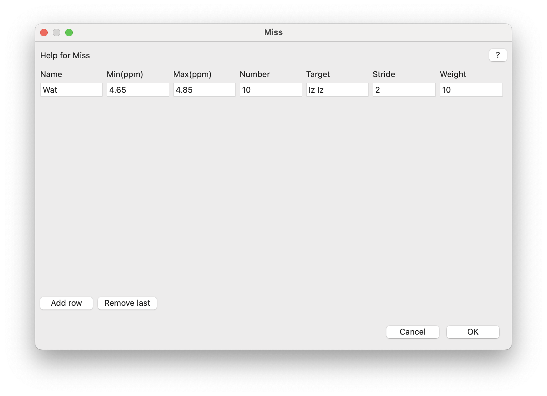
Assigns different weights to different optimisation bands when some regions are more important than others.
use only after reading the corresponding Technical Manual section or loading a template that demonstrates the mode.
Warning
Do not tune advanced controls merely because they are available. Start with the template defaults and change these options only when the problem or the report gives you a reason to do so.
The Read tab imports an existing pulse for analysis, conversion, or further optimisation. It is particularly useful when improving a previously designed pulse, comparing pulse performance, or converting between spectrometer formats. You can start the optimisation from a pulse shape that you have just read in (though we find it is usually better to start from random).
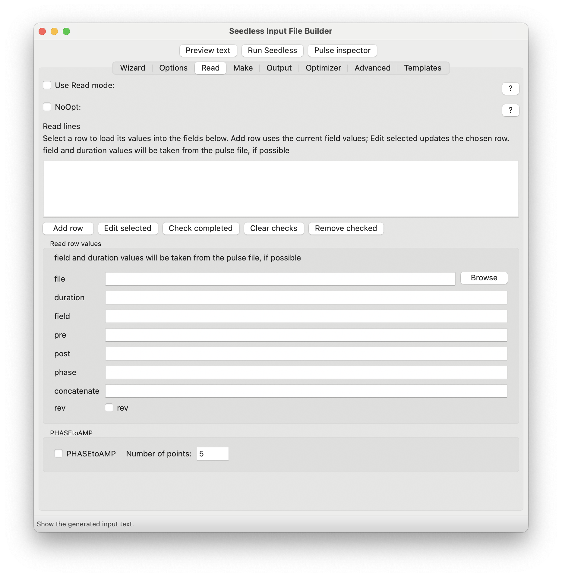
Each row may specify a file and optional overrides:
total pulse duration in microseconds;
maximum B1 in Hz;
zero-amplitude evolution before or after the pulse;
common phase shift in degrees;
number of repetitions; and
time-and-phase reversal at import.
Choose NoOpt when you wish to analyse or convert an existing pulse without performing any further optimisation. Before importing vendor-formatted pulses, verify the column layout and phase conventions on the Output tab to ensure that the pulse is interpreted correctly.
The Make tab generates standard pulse shapes directly or performs calibration and pulse-transformation operations. In contrast to the Wizard, which defines a new optimisation problem, Make mode begins from an existing analytical pulse construction or transformation. Make mode constructs standard shapes such as EBURP1, REBURP1, CHIRP, Q3, Q5, SEDUCE, HARD, TANH, and CHORUS, or performs supported calibration and transformation operations. See the examples in the Templates tab.
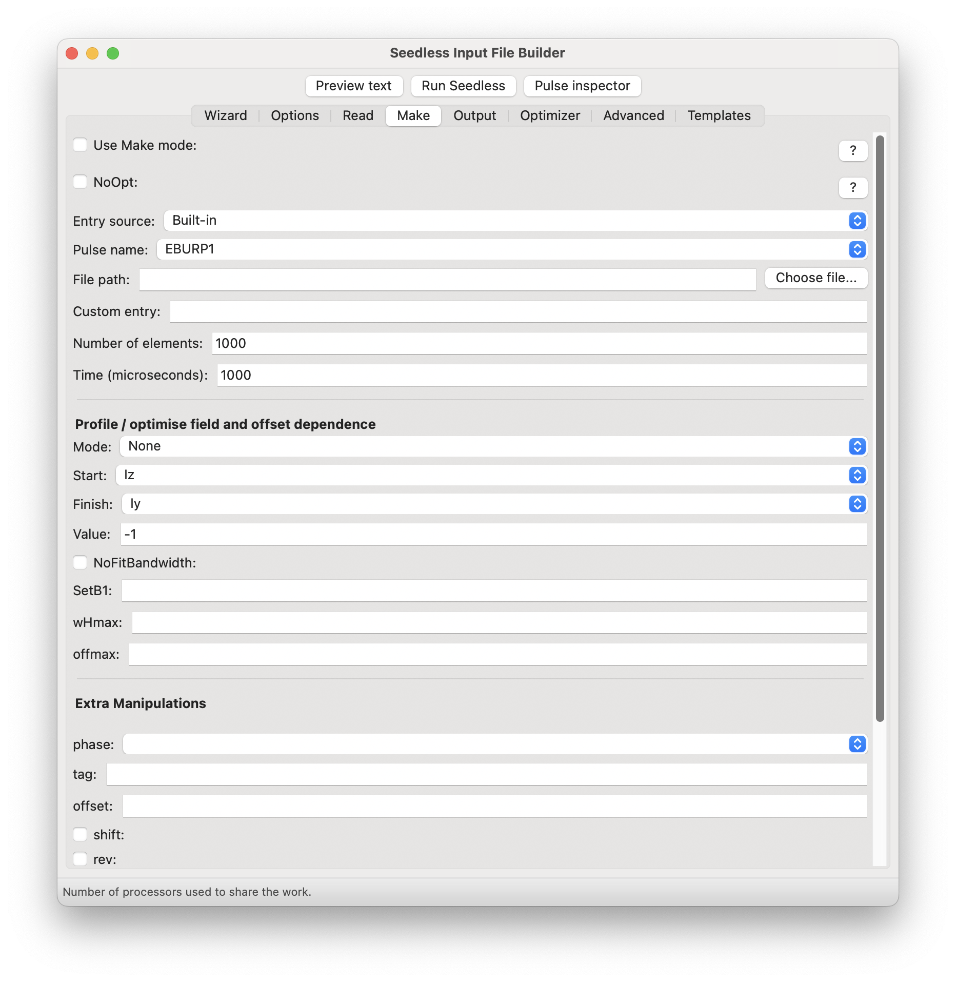
For routine GUI use:
The theory and exact syntax for transforms, adiabatic modes, and calibration are in the Technical Manual.
Warning
The Bruker flag will reverse the sign of the phases of pulses on both input and output. Do not use this for Varian or Jeol pulses. Pulse simulation software on your hardware, such as shapetool in Bruker, should show how the pulse will perform on the spectrometer.
The Output tab determines how pulses are written for the destination spectrometer. Selecting the correct convention is essential because different vendors use different phase conventions, file formats, and waveform definitions.
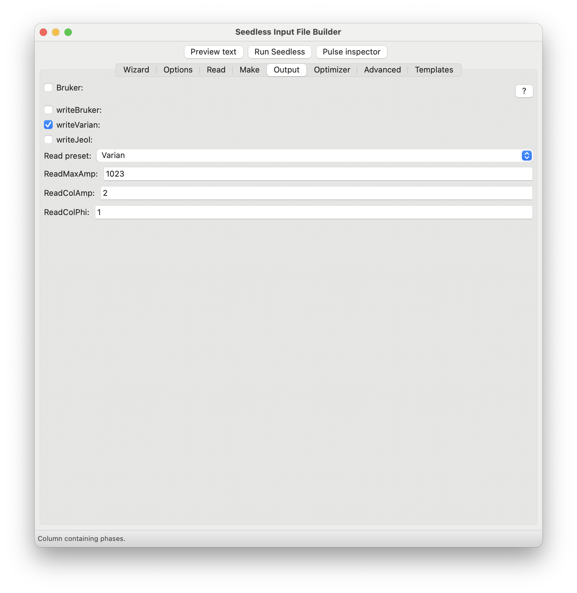
Choose the convention for the destination spectrometer before exporting or importing a shape. Treat the exported file as an instrument input: inspect it, preserve the calibration information, and validate it using local procedures.
Most users only need to adjust a small number of optimisation settings. The remaining controls can usually be left at their template defaults.
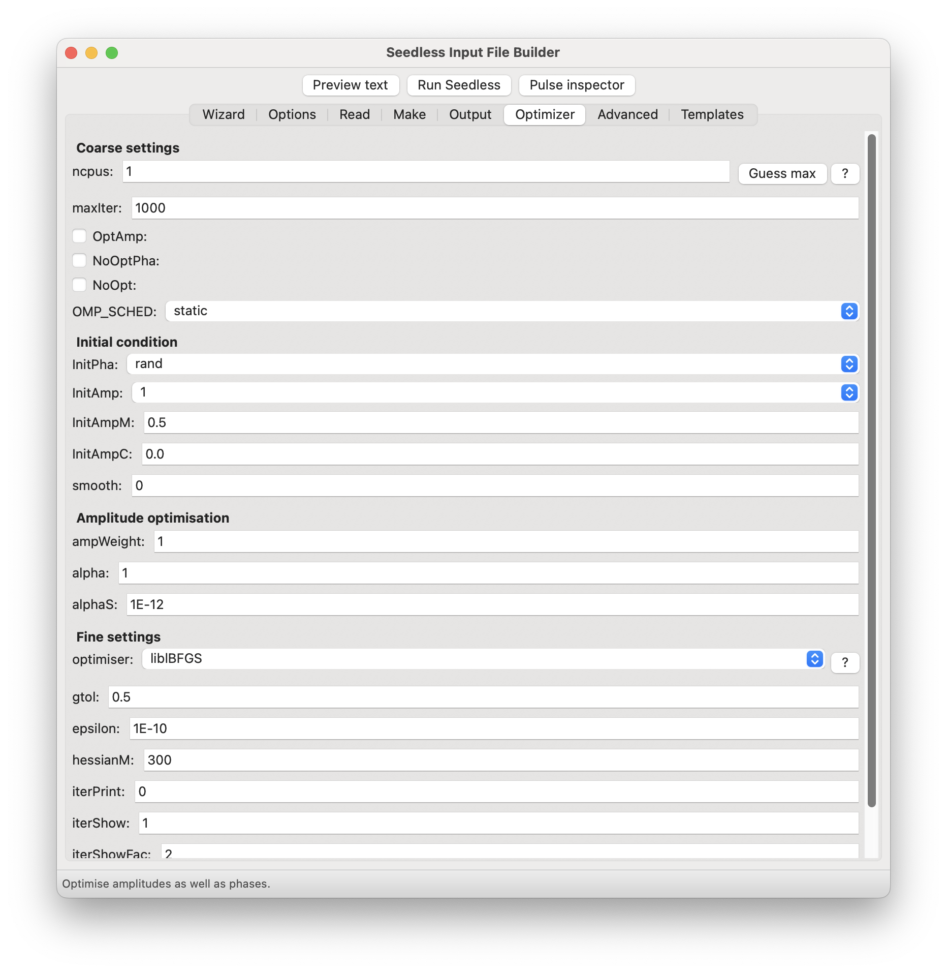
The most useful routine controls are:
number of CPU cores. Guess max chooses a reasonable detected value.
maximum optimiser iterations. A value of zero may request automatic behaviour, depending on the current program version.
normally enabled for the recommended phase-only workflow.
normally disabled unless amplitude modulation is specifically required.
control how the pulse is started, and the seed for the random number generator.
Leave tolerances and specialised optimiser settings at template defaults until the report or the Technical Manual gives a reason to change them. The default values behave well.
Practical tip
When making a new pulse, set maxIter to a relatively small number, ca. 1000. You can inspect how infidelity changes with iteration in the report. If the trend looks promising, repeat with more iterations to drive the computation towards convergence. We often stop after a few thousand iterations rather than pushing the computation to one of the convergence thresholds.
The Advanced tab collects specialised analysis and diagnostic tools that are not normally required during routine pulse design. Most users will only visit this tab when investigating optimisation behaviour or following an advanced example from the Templates tab or the Technical Manual.
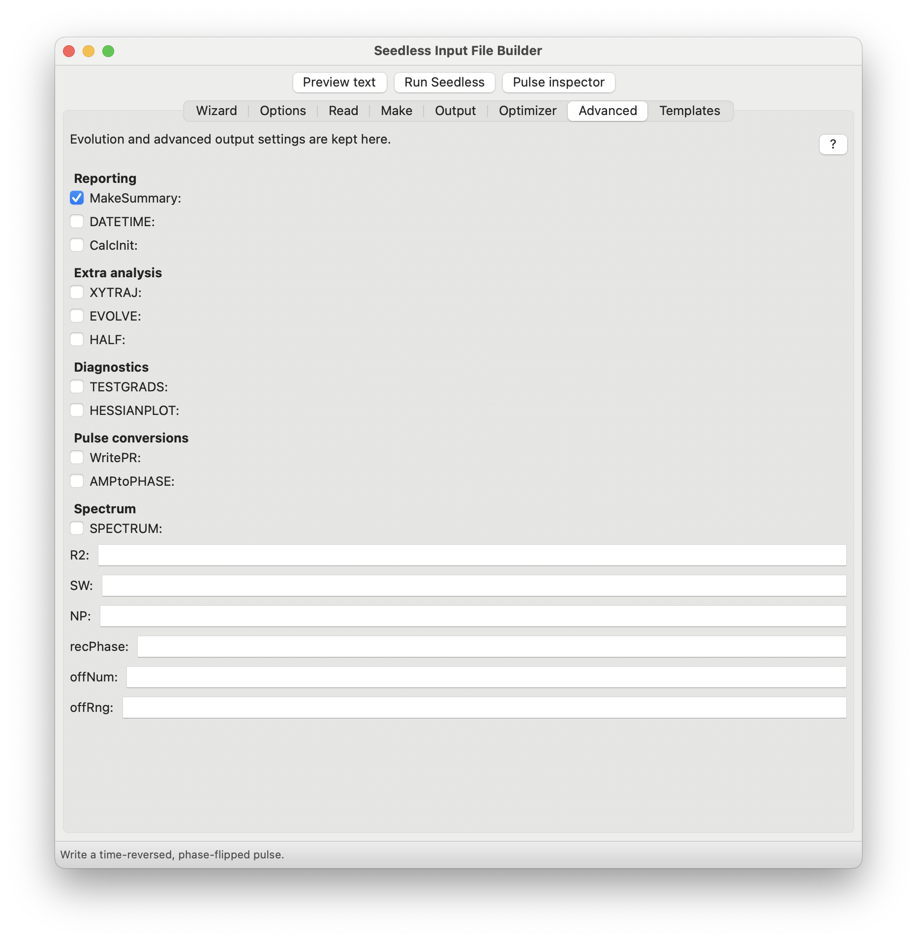
The Advanced tab groups specialised output and analysis features. Typical reasons to visit it are:
Use the question-mark help for field-level reminders and the Technical Manual for interpretation. Advanced diagnostics can be computationally expensive and may produce outputs that are not needed for routine pulse design.
Templates serve two complementary purposes. They provide validated examples of common pulse-design problems and act as reliable starting points for new optimisations. Whenever possible, begin with the template that most closely resembles the intended experiment rather than constructing a new optimisation from scratch. Double-clicking loads a template; Load selected template does the same explicitly.
After the single HNCO example in Section 4 succeeds, Run pulse collections provides a broader installation and regression test. It runs many supplied examples and reports pulse names, infidelities, and calculation times. Timings vary with computer, compiler, CPU count, and program version; compare the kinds of outputs and approximate scores rather than expecting identical times.
Successful completion of the supplied pulse collection provides confidence that the installation is functioning correctly across a wide range of optimisation modes, although small differences in optimisation time and final infidelity between computers are entirely normal.
The following workflow has proved reliable for both new and experienced Seedless users. It emphasises making incremental changes, checking the generated input before optimisation, and evaluating each optimisation systematically. Following this sequence reduces the likelihood of introducing multiple independent changes that are difficult to diagnose.
Note
The same iterative approach is recommended throughout the Seedless Technical Manual. Successful pulse optimisation is rarely achieved in a single calculation; instead, it is usually the result of a sequence of small, well-understood refinements.
Most difficulties encountered when using the Seedless GUI fall into one of three categories:
When diagnosing a problem, begin with the simplest explanation. First confirm that the installation is functioning correctly, then compare your settings with a working template, and only then begin modifying optimisation parameters. Installation and platform-specific troubleshooting are described in detail in the Seedless Technical Manual; the table below focuses on common problems encountered when using the GUI.
|
Symptom |
Likely cause |
Recommended action |
|
The window does not open |
Python, wxPython, matplotlib, path, or launcher problem |
Follow the installation checks in the Seedless Technical Manual. Verify that the same Python interpreter can successfully execute import wx. |
|
Run Seedless does nothing or reports no binary |
No matching executable, blocked permission, or incorrect installation layout |
Read the console message carefully, confirm that the correct Seedless executable exists, check file permissions, and verify that the expected bin directory is being used. |
|
The summary PDF is missing |
gnuplot or pdflatex is unavailable, or summary generation is disabled |
Test both programs from the same execution environment and confirm that MakeSummary appears in the generated Preview text. |
|
Preview text looks wrong |
One or more tabs contain incomplete, inconsistent, or stale settings |
Return to the relevant tab, check row counts, units, and entered values, then compare the generated input with a known working template. |
|
Targets do not match regions |
The number of SpinSystem regions differs from the number of optimisation targets |
Ensure that every SpinSystem region has exactly one corresponding optimisation target. |
|
The score is poor |
The requested pulse is too short, RF power is too low, optimisation regions are too wide, transition bands are too sharp, or sampling is insufficient |
Return to the nearest working template. Increase pulse duration or RF power (within safe experimental limits), relax the optimisation requirements, or investigate the design systematically using Grid Search. |
|
The score is good but the plotted profile has holes |
The optimisation sampling is too sparse |
Increase the number of optimisation samples within the SpinSystem regions and use an even denser plotting grid to verify the pulse behaviour between optimisation points. |
|
The pulse score varies with random seed |
Different random initial conditions converge to different local optima |
Fix the random seed when reproducing results or use Horserace mode to compare multiple optimisation runs. The stochastic nature of these optimisations is discussed in the Seedless Technical Manual. |
|
The experiment performs worse than the simulation |
RF calibration, pulse-format conventions, transient behaviour, duty cycle, or experimental conditions differ from the optimisation model |
Verify RF calibration, confirm that the correct vendor output format has been selected, validate the pulse on the spectrometer, and consider transient analysis if appropriate. Reducing the finite-element duration may also improve experimental performance. |
One of the strengths of the Seedless GUI is that it generates standard Seedless input files automatically. Most users can therefore design and optimise pulses without needing to learn the underlying input syntax.
The table below provides a cross-reference between the principal GUI controls and the corresponding Seedless input keywords. It is intended as a quick reference rather than a complete description of the input language. Users who wish to edit input files manually or understand the meaning of individual keywords in greater detail should refer to the Seedless Technical Manual, where every input section is described in full.
|
GUI concept |
Input keyword or section |
Purpose |
|
Nucleus frequency |
frq |
Reference frequency (MHz) for the nucleus being optimised. |
|
Maximum RF field |
wmH: |
Maximum available RF nutation frequency (Hz). |
|
RF distribution |
RF: |
Relative RF-field values and weighting used to model RF inhomogeneity. |
|
Carrier |
Carriers: |
Carrier frequencies (ppm) for one or more optimisation calculations. |
|
Validation grid |
Plot: |
Frequency grid used to evaluate and plot the final pulse performance. |
|
Optimisation bands |
SpinSystem: |
Chemical-shift regions together with the optimisation sampling density. |
|
Pulse durations |
Durations: |
Pulse durations and corresponding finite-element counts. |
|
Targets |
Targets: |
Desired pulse operation for each optimisation region. |
|
Output directory |
outPath |
Directory in which generated pulse files and reports are written. |
|
Pulse label |
pulseName |
User-defined pulse name or automatic naming convention. |
|
Random seed |
seed |
Initial random-number seed for reproducible optimisations. |
|
Summary report |
MakeSummary |
Enables generation of the PDF optimisation report. |
|
Vendor format |
Bruker, Varian, Jeol |
Spectrometer-specific output formats and phase conventions. |
|
CPU count |
ncpus |
Number of processor cores used during optimisation. |
|
Iteration cap |
maxIter |
Maximum number of optimiser iterations. |
|
Read mode |
Read lines |
Import an existing pulse for analysis, conversion, or further optimisation. |
|
Make mode |
Make commands |
Generate or calibrate built-in pulse shapes before optimisation. |
The GUI provides a convenient interface to the full capabilities of the Seedless optimisation engine. Most users will find that the Wizard and the supplied templates are sufficient for routine pulse design, while the notebook tabs provide progressively finer control as experience grows.
The recommended approach is to begin with a validated template, modify one aspect of the optimisation at a time, inspect the generated input using Preview text, and evaluate every optimisation using the Pulse Inspector and summary report.
For detailed discussions of optimisation strategy, convergence behaviour, pulse-design methodology, and the complete Seedless input language, readers should consult the accompanying Seedless Technical Manual.