|
|
|
|
Note
This guide is intended for users who want to generate shaped pulses for NMR experiments using Seedless. Please see the companion Seedless GUI Manual. This technical manual starts with the basic workflow needed to create and test a pulse, then introduces the more advanced optimisation options and practical considerations. Some familiarity with NMR pulse sequences and shaped pulses is assumed, but the early sections are written for users who have not used Seedless before.
Seedless rapidly calculates GRAPE pulses, primarily for NMR spectroscopy, and is fast enough to generate pulses matched to particular hardware and sample conditions [?, ?, ?]. Properly designed pulses can significantly improve experimental sensitivity. Its speed comes from combining established and newer optimisation ideas [?, ?]. In addition to bespoke GRAPE calculations, the program can construct and analyse traditional shapes such as BURP and CHIRP pulses, optimise smooth Fourier or power-series descriptions, import existing shapes, and perform specialised evolution and diagnostic analyses.
Pulse design is an engineering problem with competing constraints. Bandwidth, selectivity, pulse duration, maximum B1, RF inhomogeneity, finite-element duration, transition width, and required transformation all affect the attainable performance. The program makes it inexpensive to explore these compromises, but a low numerical score does not remove the need to check the full simulated profile and validate the result experimentally.
Seedless is written in C++ and controlled by a text input file. The companion GUI constructs the same file from graphical controls. This manual introduces each concept in terms of the underlying script, then retains a complete syntax reference in Section x1-570001010. The companion GUI manual focuses more on getting up and running quickly.
Seedless focuses on isolated spin-1/2 systems. When only one spin is pulsed at a time and evolution is controlled appropriately, such pulses will exactly control weakly coupled systems and to higher-spin nuclei whose anisotropic interactions are motionally averaged [?].
The recommended default is constant-amplitude, phase-only optimisation [?]. In our experience it is fast, robust, and usually performs at least as well as a comparable simultaneous amplitude-and-phase optimisation. Amplitude-only and combined modes remain available when the hardware or application requires them, as do conversions between phase-only and amplitude-modulated forms.
Otherwise, enjoy using Seedless. Please email us if you have any problems.
Andy Baldwin and Jonathan Jones
jonathan.jones@physics.ox.ac.uk
© University of Oxford
Thanks to Team Seedless: Charles Bunchanan, Gaurav Bhole, Jack Bercovici, Bowen Guo, Suzanne Lim, Abi Turner, Gogulan Karunanithy, Virginia Casablancas-Antras, Adeline Poh, Ben Davis, Eiso Ab.
The full demonstration suite provides a useful regression test once the initial example is working. It should create 36 pulses of a wide range of pulse types. You can run this from the command line, or clicking Run pulse collections in the Templates tab in the GUI.
If you can run the demonstration and you can generate the output files, the installation was successful and you are good to go.
The downloaded distribution should contain the following folders. For the initial tests, keep this directory structure unchanged, as many of the demonstration scripts locate the executable using relative paths.
| Folder | Purpose |
| bin | Seedless executables and the files needed to run them. This is the folder used when setting the executable path. |
| demo | Worked examples and scripts. These are the best starting points for testing the installation and for making new input files by editing a known working example. |
| papers | Related publications and background material. These are useful for understanding the design choices and examples, but are not required for running Seedless. |
| manual | Contains the technical and GUI manuals for Seedless, together with HTML versions that can be viewed conveniently in a web browser. |
Practical tip
For the first test, do not move files out of the download tree. Run the full demonstration suite from the original directory structure before moving or reorganising any files. Or try the GUI.
A complete installation requires:
Adding the bin folder to the system path is convenient but not required. This directory contains all binaries and supporting libraries required to run Seedless. For first tests, an explicit or relative path to the executable files is often easier to diagnose.
Installation of gnuplot and pdflatex depends on the operating system. Instructions for macOS, Linux and Windows are given.
seedless_Darwin_arm
seedless_Windows_x86_64.exe
seedless_Linux_x86_64
Use the binary that matches the system. On macOS, the first launch may require approval under Privacy &Security. On Unix-like systems, ensure that executable permission is set. On Windows a similar procedure will probably be needed to allow the system to run the binary.
====================================
 Welcome to Seedless version 1.3
====================================
 Fast optimal control pulses.
------------------------------------
                    C.Buchanan
                    G.Bhole
                    J.Jones
                    A.Baldwin
      (c) University of Oxford
------------------------------------
 Special thanks to G.Buo and S. Lim
------------------------------------
You have identified the correct binary if running it from a terminal produces the banner shown above. If you see an error, there is a compatibility problem. Work through the troubleshooting steps below and get in touch if the problem persists.
Homebrew can install reporting dependencies:
brew install gnuplot
brew install basictex
If you intend to use LaTeX, you may prefer a more complete distribution (ca. 7 Gb) rather than the basic (130 Mb) using
brew install mactex
Open a new terminal after installation, then test gnuplot and pdflatex. If you get a message from the programs, the installation was successful. Run one of the supplied demonstrations using the wrapper or an explicit binary path, for example:
python3 ../../bin/seedlessRun
../../bin/seedless_Darwin_arm seedless.C
Install gnuplot and a LaTeX distribution using the system package manager. On Ubuntu or Debian-derived systems, a typical starting point is:
sudo apt-get update
sudo apt-get install gnuplot texlive-latex-base texlive-latex-extra
Open a new terminal after installation, then test gnuplot and pdflatex. If you get a message from the programs, the installation was successful. Then run the Seedless wrapper or binary explicitly:
python3 ../../bin/seedlessRun
../../bin/seedless_Linux_x86_64 seedless.C
If you want to run Seedless from any folder, add the Seedless bin directory to your shell path. For example, in
bash you would add a line like this to ~/.bashrc, replacing the path with the actual location of your Seedless
folder:
export PATH="PATH:/path/to/Seedless/bin"
Then open a new terminal or reload the file with source ~/.bashrc.
Older Linux distributions might fail to run seedless_Linux_x86_64, reporting that libmvec is not
present. We have included an additional binary seedless_Linux_x86_64_OLD. If you encounter this error, go
to the bin folder and run
cp ./seedless_Linux_x86_64_OLD ./seedless_Linux_x86_64
This replaces the default binary with one compiled without libmvec. Thanks to Eiso Ab for figuring this out.
On Windows, install Seedless, Gnuplot, and a LaTeX distribution that provides pdflatex.
Install Gnuplot from SourceForge: https://sourceforge.net/projects/gnuplot/files/gnuplot/
Install pdfLaTeX using either TeXLive or MiKTeX.
After installation, check that the following folders are on your Windows Path. The exact locations will
depend on where you installed each program:
C:\Program Files\gnuplot\bin;
C:\texlive\2025\bin\Windows;
bin folder, for example C:\path\to\Seedless\bin.To edit your user path on Windows:
Edit environment variables for your account.
User variables, select Path and click Edit. If Path does not exist, create it.
bin folder, the LaTeX bin folder, and the Seedless bin folder.
gnuplot and pdflatex.There are two Windows environment-variable editors: one for your user account and one for system-wide variables. Editing the user account path is sufficient, which usually does not require administrator access.
Open a new terminal after installation, then test gnuplot and pdflatex. If you get a message from the programs, the installation and setting of the path was successful. To run Seedless directly on Windows, open a terminal in the folder containing the input file and use:
seedless_Windows_x86_64.exe seedless.C
if the Seedless bin folder is on the path. Otherwise, call it using the full or relative path to the
executable.
To use seedlessRun on Windows, Python must also be installed and visible on the path. Then
run:
python seedlessRun
from a suitable folder, or call seedlessRun using its full path.
Install the GUI dependencies into the same Python environment that launches seedless_gui. This is the same on all platforms:
python3 -m pip install --upgrade pip
python3 -m pip install --upgrade matplotlib wxPython
python3 -c "mport wx; import matplotlib; print(wx.version())"/span>
If the final step gives an error, then wxPython has not installed correctly. The companion GUI manual begins after this import test and the platform binary test succeed. Launch the GUI with
seedless_gui
Or supply the path if the bin folder is not in the path.
There are three options. The following examples assume that the bin directory is on your system path. If it isn’t, you will need to type in the path before the commands.
seedlessRun
recursively locates inputs whose names begin with seedless, runs them in their home folders, and writes a consolidated report. It is convenient for demo suites and batches.
For development and debugging, it is often preferable to invoke the binary directly. This gives the clearest terminal diagnostics while developing a new pulse:
seedless_Platform_Chipset inputfile
Chosen from the list
seedless_Darwin_arm
seedless_Windows_x86_64.exe
seedless_Linux_x86_64
Alternatively, launch the GUI using
seedless_gui
seedlessRun and seedless_gui are executable python scripts. You may need to make them
executable with e.g. chmod +x seedlessRun (macOS and Linux). You can also launch them
with
python3 seedlessRun
python3 seedless_gui
The header command MakeSummary enables a PDF report. Report generation requires gnuplot and pdflatex. Test both from the same terminal or environment used to run Seedless before changing the pulse input.
If you run into trouble, the most likely cause is the installation. Find a friendly local IT person, ask Mr. Google or your favourite AI for help.
The quickest way to learn Seedless is not to begin with a blank input file, but with a calculation that is already known to work. Throughout both the GUI and technical manuals we therefore use the same canonical example: an 80 μs 13C excitation pulse for an HNCO experiment. The pulse performs three different tasks simultaneously:
Although relatively simple, this example illustrates nearly every important idea in Seedless: multiple chemical-shift bands, different restraints in different regions, RF inhomogeneity, finite-element optimisation and validation with a summary report.
Before writing a single line of syntax, it is helpful to think like a pulse designer. Ask four questions.
For this HNCO example the answers are straightforward.
The pulse belongs to a triple-resonance experiment. Only three carbon bands are important (CO, Cα, and Cβ). CO must be excited, whereas the remaining two bands should behave as spectators. A pulse duration of 80 μs and a maximum RF field of 17.6 kHz are realistic on many modern probes and provide an excellent demonstration problem.
Only after these experimental decisions have been made do we describe them using Seedless syntax.
ncpus 8
frq 150
outPath ./HNCO/C/
maxIter 5000
MakeSummary
Bruker
RF:
  0.93 0.25
  1.00 0.50
  1.05 0.25
Plot:
  P 0 200 360
SpinSystem:
  CO 165 185 96
  CA 40 78 96
  CB 8 40 96
Carriers:
  176
wmH:
  17605
Durations:
  80E-6 80
Targets:
  Iz -Iy , Iz Iz , Iz Iz
Rather than trying to memorise the individual keywords, read the file from top to bottom as a description of the experiment.
defines the spectrometer, output files and optimisation.
specifies the RF inhomogeneity distribution.
defines the dense validation grid used after optimisation.
defines the three chemical-shift bands.
places the RF carrier at 176 ppm.
sets the maximum RF field.
specifies the pulse duration and number of finite elements.
specifies the desired transformation in each band.
Notice that the input file never tells Seedless how to produce the pulse. Instead it describes what the pulse should achieve. The optimiser is responsible for finding a pulse that satisfies those constraints.
Practical tip
Read every Seedless input file as a scientific description of the pulse rather than as a computer program.
While learning Seedless, we recommend running the platform binary directly, for example
../../bin/seedless_Darwin_arm seedless.C
or the corresponding Linux or Windows executable. The GUI writes exactly the same input file before launching the calculation. Understanding this relationship between the GUI and the underlying input file makes it much easier to move confidently between the two interfaces.
Warning
If no summary PDF is produced, the optimisation may still have succeeded. The most common cause is that gnuplot or pdflatex is not available on the system path.
The exact pulse phases differ slightly between computers because the optimisation begins from random initial conditions. Do not expect the pulse shape itself neccessarily to be identical. Instead check that
If these points agree with the supplied example then your installation is working correctly. The next section explains how to interpret the summary report and assess whether a pulse is suitable for experimental use.
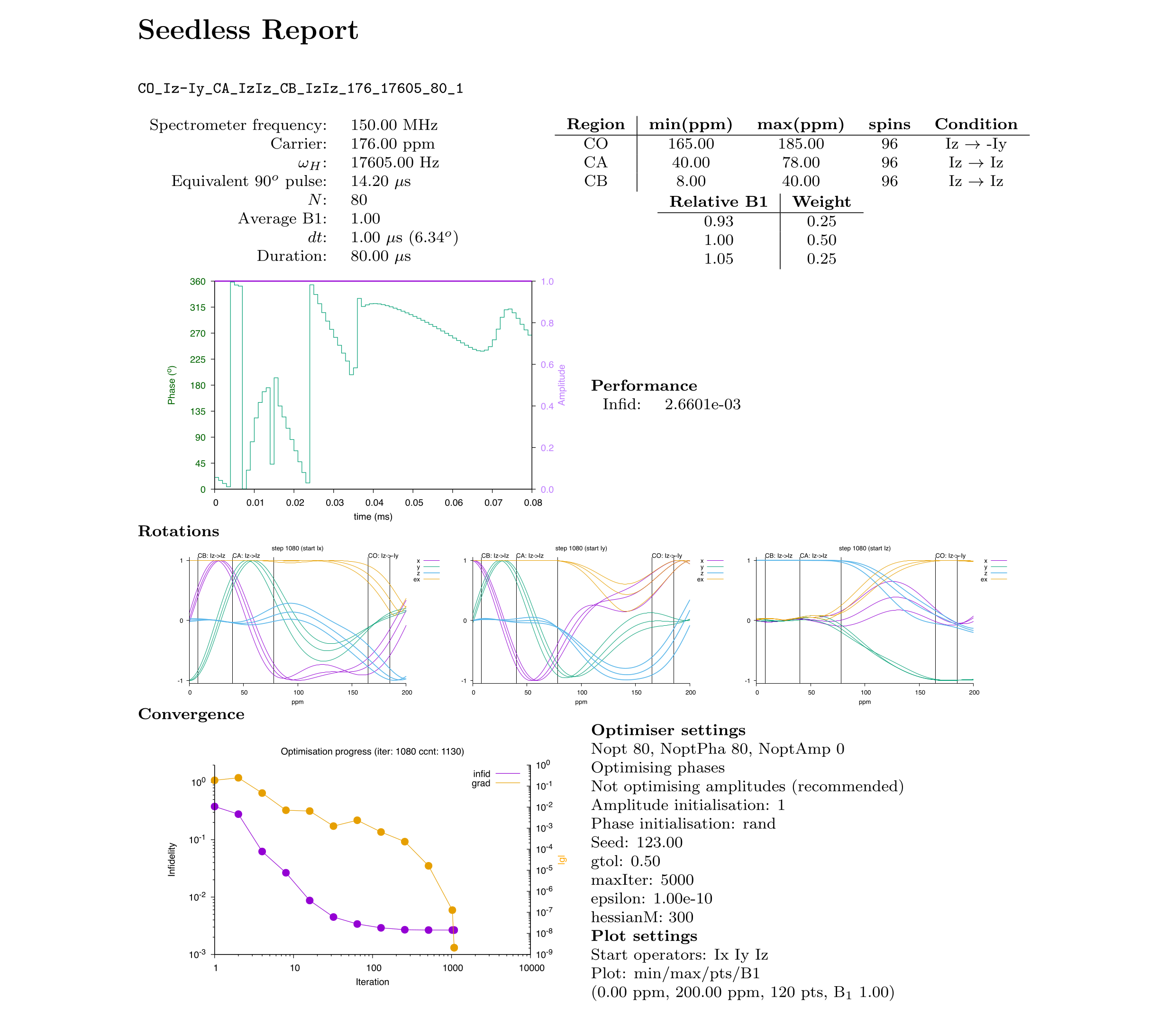
If MakeSummary is included in the input file, and both gnuplot and pdflatex are available, Seedless produces a PDF report summarising both the optimisation and the behaviour of the final pulse. The report is much more than a record of the calculation. It is the primary tool for deciding whether a pulse is ready for experimental use. An experienced pulse designer rarely studies the report from top to bottom. Instead, it is best viewed as a sequence of diagnostic questions.
Whenever you calculate a new pulse, work through the following checklist.
Working through the report in this order usually identifies problems much more quickly than looking only at the final infidelity.
Begin with the summary at the top of the report. Confirm that
Many apparently poor optimisations are simply the result of calculations performed using incorrect input parameters.
Warning
Always check the report before examining the pulse. An optimisation can be excellent while solving the wrong problem.

The rotation plots are the most important part of the report. Each panel begins with magnetisation aligned along one of the Cartesian axes (Ix, Iy or Iz) and shows where that magnetisation finishes as a function of chemical shift. Remember that only restrained transformations are expected to look simple. For the HNCO example the targets are
CO: Iz →−Iy
CA: Iz → Iz
CB: Iz → Iz
Therefore the Iz plot is the principal figure of merit. The behaviour of magnetisation that starts along Ix or Iy was never restrained and may appear complicated. This is entirely normal for a state-to-state pulse. By contrast, a universal 90x pulse should show the expected behaviour for all three starting axes.
Practical tip
Judge the pulse only against the restraints you actually requested.
Seedless optimises only the frequencies supplied in the SpinSystem: section. The plotted report is evaluated on a denser plotting grid to make sure performance is good for all frequencies within the band. Inspect the Rotation plots carefully.
If not, increase the optimisation sampling, perhaps make the pulse duration longer, and repeat the calculation.
Why this matters: A pulse that performs perfectly at optimisation points can still perform poorly between them.
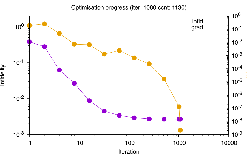
The convergence plot shows the infidelity and gradient as a function of iteration. In this case, the pulse met its ‘true’ convergence after 1080 iterations. Reaching this point required 1130 calls to the expensive ‘compute infidelity and gradients’ function.
During the first few hundred iterations the infidelity typically decreases rapidly. Thereafter the curve begins to plateau. The optimiser, however, continues refining the pulse, often smoothing the waveform while making progressively smaller improvements to the cost function. The gradient norm, |g|, typically decreases approximately exponentially throughout the optimisation.
A convergence curve that has the infidelity still falling steeply usually indicates that the optimisation was stopped too early. A flat infidelity curve may indicate
Practical tip
Interpret the convergence together with the rotation plots.
Finally, ask whether you would actually use this pulse. Consider
Only after answering these questions does it become meaningful to compare infidelity values between different pulses.
There is no universal numerical threshold. For many applications when considering the infidelity
10−4 or below : excellent
10−3 : very good
10−2 : can be usable for difficult problems
These values are only guidelines. Transition bands are intrinsically difficult. If two different restraints are required close together in frequency compared with the inverse pulse length then the behaviour at the boundary will be hard to control. A relatively high overall infidelity may simply reflect a difficult transition region, the pulse may still perform well in the bands that matter experimentally. Similarly, water-miss pulses often produce larger infidelities while still giving reasonable experimental performance reflecting the challenge of reconciling conflicting restraints.
Ultimately, the experiment is the final judge. In the words of Lewis Kay,
The spectrometer never lies.
If you get increased sensitivity or better selectivity in a spectrum, you have a good pulse.
The next chapter describes how to improve a pulse systematically once the report has identified its strengths and weaknesses.
Designing a pulse is fundamentally an engineering problem. Before writing a Seedless input file, you need to decide exactly what the pulse must do, which compromises are acceptable, and what limitations are imposed by the spectrometer. Every successful Seedless calculation begins by answering four questions:
Once these questions have been answered, the Seedless syntax simply becomes a way of describing those decisions. The detailed syntax is collected later in Section x1-570001010.
When designing a new pulse we recommend the following order:
A useful principle is to change only one design variable at a time. If the pulse is too long, reduce the duration. If the quality is poor, increase the duration and B1. If the pulse is still unsatisfactory, reconsider whether the requested restraints are stricter than the experiment actually requires.
The virtual spectrometer describes the experimental environment in which the pulse will operate. The aim is not to reproduce every detail of the hardware, but to capture the quantities that determine pulse performance. Modern NMR spectrometers generally reproduce these in silico simulations remarkably well, particularly when the finite-element duration is several hundred nanoseconds or longer.
The most important experimental parameter is the calibrated RF field. Measure the 90∘ pulse length t90 for the nucleus of interest and calculate

Use the highest RF field that your probe can safely sustain for the intended pulse duration. Modern probes are often capable of operating at their maximum calibrated field for several hundred microseconds. If the desired pulse requires a substantially longer duration, reduce the RF field so that the duty cycle remains within the manufacturer’s recommendations.
Practical tip
Choose the highest safe RF field first. It is usually easier to increase the pulse duration later than to recover performance from an unnecessarily weak RF field.
Warning
Always check the RF and duty-cycle limits of your probe and spectrometer to ensure that pulses are neither designed nor tested outside the recommended operating conditions. Note that the power goes with ν12, so halving the B1 reduces the power requirements by 4. At this reduced power level, spectrometers can usually pulse for milli-seconds. For solution NMR we routinely apply pulses for hundreds of μs at maximum amplifier power.
Corresponding syntax: wmH: (Section x1-8100010.4.510.4.5).
Real samples experience a distribution of RF fields rather than a single value. Seedless therefore optimises the average performance across a distribution of relative RF amplitudes.
A simple three-point model is usually an excellent starting point. It improves robustness without making the optimisation unnecessarily expensive. The B1 inhomogeneity can be measured by Fourier transforming the nutation curve or visualised using an imaging experiment [?].
Practical tip
Do not optimise only for the centre of the sample if the pulse will be used over the whole active volume. The three-point distribution has worked extremely well for us over a wide range of NMR hardware.
Corresponding syntax: RF: (Section x1-7700010.4.110.4.1).
A shaped pulse is represented as many short hard pulses (finite elements). Increasing the number of finite elements allows increasingly complex pulse shapes, but also increases optimisation time and makes the pulse more sensitive to hardware transients. For most liquid-state applications, element lengths of roughly 1–2 μs provide an excellent starting point.
To estimate the total duration (T), the product B1T provides a useful guide. Pulses created with the same restraints will often have a similar infidelity for a range of durations provided the product stays constant. As a useful rule of thumb, B1T >10 usually gives the optimiser sufficient freedom to satisfy the required controls.
Practical tip
Once a satisfactory pulse has been obtained, increase the finite-element length until performance begins to deteriorate. This will produce a pulse that is easier for the spectrometer to reproduce faithfully.
Corresponding syntax: Durations: (Section x1-8200010.4.610.4.6).
The optimisation grid defines the frequencies used while designing the pulse. The plotting grid is different: it is a validation grid used to test the finished pulse between optimisation points.
Always validate on a denser grid than was used for optimisation.
Practical tip
A pulse should perform well not only at the frequencies it was optimised for, but also between them. As a general guide, use a plotting density three to four times higher than the optimisation density.
Corresponding syntax: Plot: (Section x1-7800010.4.210.4.2).
The most important design decision is not the optimiser, but the restraint. Always ask: what does the experiment actually require?
If only one initial state is ever present experimentally, there is usually no advantage in demanding a full unitary rotation and a state-to-state pulse can be used instead. As this is a less demanding pulse, it can be shorter.
Universal: should be reserved for pulses that must handle many different coherence pathways and starting states.
State-to-state: if the pulse sequence only needs a single transform. Requires less time/power than universal.
XYcite: a special case of state-to-state transfer. They move magnetisation into the transverse plane with uncontrolled phase. These pulses are often very short, but the phase is not ordered. These can be used in symmetric pairs to compensate for variable evolution with frequency (ppm).
Evolution: these control the duration for which chemical shift and scalar coupling are active in a pre and post evolution periods that flank a ‘zero time’ central rotation[?]. There are state-to-state and unitary versions of these pulses, which are relatively demanding.
Practical tip
Choose the simplest restraint that correctly describes the experiment.
The following table gives some typical situations, and examples can be found in the demo.
| Use case | Typical target | Typical application |
| Excitation | Iz -Iy | Takes equilibrium (Z) and creates transverse phase ordered state. |
| Inversion | Iz -Iz | For decoupling or INEPT transfers on the passive spin. |
| De-excitation | Iy Iz | Return to Z at the end of a transverse period. |
| Refocusing | 180x | Needed for spin echoes, including for transverse spin in an INEPT. Does not control evolution. |
| Identity | id | Returns magnetisation in the same state as it started. For a spin evolving in an indirect dimension while ‘buying time’ for simultaneous decoupling. |
| Unitary 90 | 90x | Perform a 90∘ rotation, needed when there are multiple coherences that need to be handled simultaneously. |
| XYcite | Iz Iex | Bring magnetisation into the transverse plane as quickly as possible, but unordered. |
| REBURP | 180x
+
| A refocusing 180∘ pulse that allows scalar-coupling evolution in the pre and post regions, set by evAlpha. |
| Schematic 90 | a90xb / Iz -0.5OIy | The evolution delays are set by evAlpha and evBeta for the former, the second state-to-state controls explicitly controls only the post evolution. |
As a worked example, here is the pulse selection logic for a sensitivity enhanced HSQC.
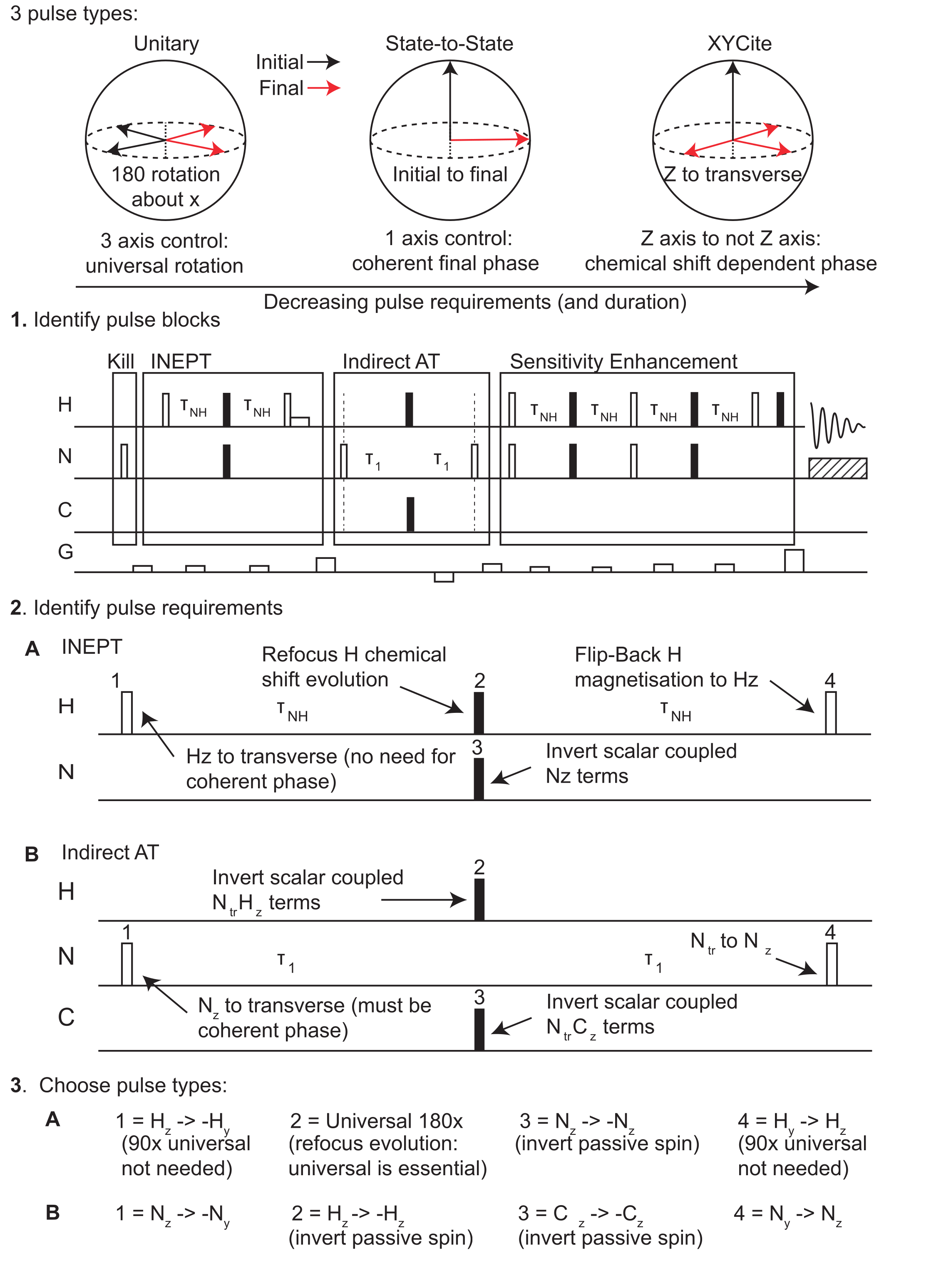
Some experiments need the pulse to do more than produce the right final state; they also need the pulse to control how much chemical-shift and weak-scalar coupling evolution takes place during the pulse[?]. In Seedless these are evolution-controlled or schematic pulses, and they sit naturally alongside the universal and state-to-state restraints above. The pre- and post- fractional evolution periods need to be specified.
There are two main forms.
a90xb where the fractional pre and post
evolution delays are set with evAlpha and evBeta, and using 180x with the REBURP flag, an evolution
controlled refocusing 180 can be created where evAlpha sets the evolution fraction, and evBeta
should be set to zero (section Section x1-520009.59.5).
Iz -0.5OIy (section 9.5). Here the ‘pre’ evolution delay is
uncontrolled, but the ‘post’ fractional evolution delay is explicitly fixed to 0.5. When using these modes, the later schematic-analysis keywords, EVOLVE and HALF can be used to verify if
the pulse behaves as required.
Practical tip
If the pulse must preserve the timing of refocusing or J evolution in the sequence, consider an evolution-controlled restraint early rather than trying to patch the problem later.
Corresponding syntax: Targets: (Section x1-8300010.4.710.4.7), and the schematic-analysis
keywords in Section x1-7000010.2.1110.2.11. These include a detailed custom syntax for supplying
restraints both state-to-state and universal with and without evolution control in a very general
form.
For all routine calculations we recommend constant-amplitude, phase-only optimisation. The default settings for the optimiser are typically excellent. If performance is poor, re-consider your design. Instead, first reconsider the
It is helpful to set maxIter to something relatively small, ca. 103 that gives a quick computation, letting you get close to the smallest possible infidelity, so you can inspect the results. A setting of 105 is typically required to get to the default convergence (difference in infidelity between iterations of 𝜖 = 10−10). This is not often necessary, and simply a low infidelity is sufficient for excellent performance on the spectrometer.
We have included modes to convert phase-only to amplitude/phase modulated pulses which can lower the overall integrated B1 (section Section x1-550009.89.8) [?].
Practical tip
Optimise the pulse, avoid trying to optimise the optimiser.
Do not judge a pulse from the final infidelity alone. Instead work through the report in the following order:
An infidelity near 10−4 is excellent for many applications, while 10−3 is often entirely satisfactory. Ultimately the experimental result is the final judge. Remember the words of Lewis Kay:
“The spectrometer never lies.”
Once you have calculated the first demonstration pulse successfully, the next objective is not to learn every Seedless keyword. Instead, the goal is to develop an intuition for pulse design. The supplied demonstrations are arranged so that each introduces one or two new ideas while reinforcing concepts encountered earlier.
This chapter suggests a progression that has worked well for new users. By changing only one aspect of a calculation at a time, it becomes much easier to understand why a pulse improves or deteriorates.
Begin by calculating the canonical HNCO pulse described in Section x1-1400055. Do not modify the input file. Your objective is simply to confirm that
Practical tip
Never begin learning by writing a completely new input file. Start from a working example and understand why it works.
Copy the example input and modify a single quantity. Useful first experiments include
After each change, inspect the report and ask why the pulse improved or performed worse. The objective is to build intuition rather than to produce an optimal pulse.
Warning
Changing several parameters simultaneously makes it almost impossible to understand which design decision affected the result.
Once you are comfortable changing experimental parameters, begin changing what the pulse is actually asked to do. For example
These exercises quickly demonstrate that the requested transformation often has a much greater influence on pulse quality than optimiser settings.
Practical tip
When a pulse seems difficult, first ask whether the restraint is more demanding than the experiment really requires.
After working through several supplied examples you should begin creating your own pulses.
A useful checklist is
This is the same design philosophy discussed in Section x1-2800077.
Only after the basic workflow has become familiar is it worth exploring the advanced optimisation modes described later in this manual.
Examples include
These tools are extremely useful, but they are intended to address specific design problems rather than replace good pulse-design practice.
The demonstration directory provides examples covering a wide range of applications.
| Demo | What it demonstrates | Use it for |
| first | Simple proton universal 90-degree pulses | Practise editing a simple input file after installation. |
| HNCO | Carbon, nitrogen, and proton pulses | Examples for triple-resonance pulse design. |
| HNCA | More complex carbon targets | Multi-band target choices. |
| 19F | Ultra-broadband universal pulses | Broadband pulse design. |
| Sim | Read and analyse | Take an existing shape, find the required B1. |
| water | Excitation plus water-preservation restraints | Competing restraints and use of Miss mode. |
| Calibrate | Built-in shapes in Make mode | Shape calibration and comparison. |
| BIP | Horserace and grid-search examples | Illustrates the use of Horserace mode to avoid false minima. |
| a90x / multiSpin | Evolution-controlled pulses | Allow evolution during the pulse so the pulse sequence can be shortened. |
| newEBURP | Fourier-series construction | Demonstrates smooth series optimisation by recreating the original EBURP pulse. |
Rather than working through these in numerical order, follow the learning stages described above. Each example introduces a new design concept while reinforcing the previous ones.
Practical tip
The GUI exposes all of these examples in the Templates tab. Use the GUI manual for the loading and inspection workflow; return here for the theory and exact commands.
After the first example works, run the full supplied demo suite as a regression test. To do this, go to the
demo folder and run RunMe.sh. This will loop over all examples creating 36 pulses, and generate a report
summarising details and timings.
Calculation times vary strongly with hardware, compiler, CPU count, and program version, so compare the expected files and broad score ranges rather than exact timings.
Before moving on to the advanced chapters, you should be comfortable with the following principles.
Once these ideas become familiar, the advanced optimisation modes in the following chapters become much easier to understand because they solve specific design problems rather than introducing entirely new concepts.
This section brings together features that become useful once the basic input-file workflow is familiar. Some are routine pulse-design tools, others are primarily diagnostic, and several occupy the space between. The boundaries are not rigid: a single calculation may move naturally from pulse design to analysis, conversion, and back again. Table 1 provides a practical guide to when each feature is most useful.
| Feature | Use it when | Main commands |
| Horserace | Different random seeds give noticeably different final infidelities. | Horsey, HorseyIter, HorseyBins |
| Grid search | You need to choose sensible values for B1, pulse duration, or finite-element length. | Grid commands |
| Jiggle | A difficult optimisation may be stuck in a local minimum. | JIGGLE and Jiggle... commands |
| Amplitude optimisation | You deliberately want amplitude-only or amplitude-and-phase modulation. | OptAmp, NoOptPha |
| Evolution-controlled pulses and schematic evolution analysis | You need to design or inspect pulses that control effective evolution during the pulse. | EVOLVE, HALF, REBURP |
| Series modes | You want to optimise a smooth Fourier- or power-series representation. | SERIES commands |
| Diagnostics and conversion | You want to inspect minima or convert between phase-only and amplitude-modulated forms. | HESSIANPLOT, AMPtoPHASE, PHASEtoAMP |
| Alternative optimisers | You want to compare optimiser behaviour. | optimiser |
Practical tip
For routine NMR pulse design, start with phase-only optimisation at constant amplitude. It
is fast, robust, and gives excellent performance. You can convert the phase-only pulse to an
amplitude/phase mode later using PHASEtoAMP if you need to. Treat the more specialised modes
below as tools for diagnosis, exploration, or unusual hardware constraints.
Warning
The categories in Table 1 are guides rather than hard boundaries. For example, a feature may help both with pulse creation and with later analysis of the same pulse.
In some examples, changing the random seed can produce slightly different pulses. The spread between the best and worst final infidelities is usually modest, often around a factor of three. This mostly occurs for pulses with already low infidelities, below about 10−3, where the differences are unlikely to create visible sensitivity differences in spectra. Even so, it is undesirable for the result to depend noticeably on the seed.
A practical test is to run with Horsey set to 100, with HorseyIter set to 1000 or some other large
number sufficient to come close to convergence. This will start 100 independent calculations that proceed for
the specified number of iterations, with each starting from a different random seed. A histogram is produced
in the report that shows the distribution of solutions. If there is a spread of values, the optimiser has a risk of
finding false minima, and the problem needs a horserace. Here, only the seed that led to the best
performance is retained and run to completion. Add the following lines to the header of the input
file:
Horsey 50
HorseyIter 100
HorseyBins 10
The report adds a plot of infidelity versus iteration for the different seeds, together with a histogram showing the spread of final infidelity values from the race.
| Command | Meaning | Typical value |
| Horsey | Number of random seeds, or “horses”, to test. | 10–50 |
| HorseyIter | Number of iterations used for each seed before selecting the best one. | 20–100 |
| HorseyBins | Number of bins in the final histogram of race outcomes. | 10 |
This makes the optimisation extremely robust. For example, if 4 out of 100 random seeds
are poor, the probability that all H horses are poor is approximately (0.04)H. With H = 50,
this is astronomically small with a failure rate of 1 computation in 107. In practice, Horsey 10
with HorseyIter 20 is often enough; Horsey 50 with HorseyIter 100 is a more conservative
setting.
|
|
The BIP example illustrates the output. The left plot shows that the early trajectories for different seeds
follow different paths, and the best seed may not be obvious until convergence begins to stabilise. In this
example, seed 39 was best, but that was not apparent until about iteration 50. The right plot shows the
distribution of final infidelities. For this pulse, omitting horserace mode can lead to final infidelities that vary
by about a factor of three. The best pulses for this problem have time symmetry. By formally
imposing this symmetry with the SYM flag in the header, the false positive rate is dramatically
reduced.
The BIP demonstration includes an example of horserace mode.
Practical tip
If the best pulse solutions end up with symmetry, then enforce it during the calculation. For
broadband inversion pulses (BIPs), convergence is often significantly improved by using the
time-reversal symmetry flag SYM. The horserace can still find good solutions without this, but
symmetry gives the optimiser an easier problem.
When designing a new pulse, a common first question is: what RF field strength, pulse duration, and finite-element length are needed to reach the desired infidelity? Grid search is intended to answer this practical question before investing time in a full optimisation.
A grid search is enabled in the header of the input file. For example:
Grid Iter 1000
Grid Show 5
Grid T 5 50E-6 3E-3
Grid dt list  500E-9 1E-6 2E-6
Grid B1 list 20000  10000 5000
The three-number form, such as Grid T 5 50E-6 3E-3, is interpreted as the number of points, the minimum
value, and the maximum value. The keyword list means that all following values are read literally as the set
to test.
| Command | Meaning | Example |
| Grid Iter | Maximum number of optimisation iterations for each grid point. | Grid Iter 1000 |
| Grid Show | Iteration interval used when plotting trajectories. | Grid Show 5 |
| Grid T | Pulse durations to test. A three-number form means number, minimum, maximum. | Grid T 5 50E-6 3E-3 |
| Grid dt list | Explicit list of finite-element durations to test. | Grid dt list 500E-9 1E-6 2E-6 |
| Grid B1 list | Explicit list of RF field strengths to test, in Hz. | Grid B1 list 20000 10000 5000 |
| Grid Nmax | Skip grid points with too many finite elements. | Grid Nmax 50000 |
| Grid B1T | Loop over specified values of the product B1T. | Grid B1T log 20 3 100 |
| Grid flip | Loop over finite-element flip angles, in degrees. | Grid flip 1 5 10 |
The summary report shows optimisation trajectories and summary plots, including infidelity versus
duration and infidelity versus B1T. RF field is indicated by colour, while finite-element length is indicated by
marker type. If the trajectories are still decreasing strongly at the end of the grid run, the grid calculation
has not converged and Grid Iter should be increased.
A useful rule of thumb is that performance often begins to improve much more slowly once B1T is greater than about 10. In many examples, the final infidelity follows an approximately linear trend in log–log space:
log(final infidelity) = a log (B1.T) + b
final infidelity = c (B1.T)^a
The constants are application dependent. The practical implication is that decreasing B1 can often be compensated by increasing the duration T, provided the product B1T remains similar. This is useful when the maximum RF field is limited by the probe or by sample heating.
Warning
Grid searches can be expensive because they run many optimisations. Long durations combined
with short finite elements produce very large numbers of pulse elements. Use Grid Nmax to skip
cases that would be unnecessarily slow.
The BIP demonstration below tests five durations between 50 μs and 3 ms, three finite-element durations, and three B1 values.
|
|
The left plot shows that higher B1 and longer duration improve the pulse. The right plot shows that, for the 10 and 20 kHz fields, the points largely fall on a line when B1T is plotted against infidelity in log–log space. If the target is an infidelity below 10−4, the example suggests that B1T ≈ 10 is sufficient: approximately 500 μs at 20 kHz, 1 ms at 10 kHz, or 2 ms at 5 kHz. In this case, finite-element durations of 500 ns, 1 μs, and 2 μs give similar results.
A second type of grid search explores B1T and finite-element flip angle directly:
Grid Iter 1000
Grid Show 5
Grid Nmax 50000
Grid B1 list 10 100 1000 10000
Grid B1T log 20 3 100
Grid flip 1 5 10
Here, Grid Nmax sets an upper limit on the number of finite elements. Grid points exceeding
that limit are skipped. The Grid B1T and Grid flip commands make the grid search loop over
specified values of B1T and finite-element flip angle. This often gives intuitive plots of pulse
performance.
The example below is for a universal 180x pulse with time-reversal symmetry, designed over ±10 ppm for protons at a 1 GHz Larmor frequency. It compares finite-element flip angles of 1∘, 5∘, and 10∘, RF fields of 10, 100, 1000, and 10,000 Hz, and B1T values from 3 to 50.
For B1 = 10 kHz, the pulses are good from B1T = 3 upwards. At 1 kHz, the pulses are good provided B1T >30. At 100 Hz, excellent pulses can still be made if the flip angle is small, for example 1∘. At 10 Hz, the pulses are poor.
To design a final pulse with infidelity below 10−3, this grid suggests B1T ≈ 30 for fields below 10 kHz, or about 8 at 10 kHz. Thus, a 1 kHz pulse with B1T = 30 requires a 30 ms duration, whereas a 10 kHz pulse with B1T = 4 requires 400 μs. The finite-element duration can be estimated from the finite-element flip angle:
| (1) |
For a 10∘ finite-element flip angle, this gives approximately 27 μs at 1 kHz and 2.7 μs at 10 kHz. The number of finite elements is
| (2) |
which gives 1080 and 144 elements for the 1 and 10 kHz pulses respectively. These grid calculations are run only to 1000 iterations, so the final full optimisation is expected to improve on these values.
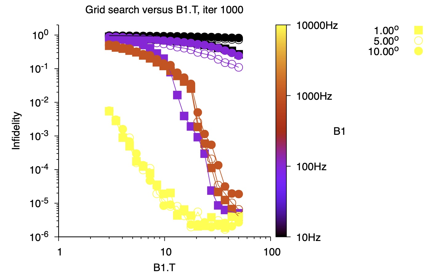
The interpretation of a plot like this is straightforward. Choose a target infidelity, read off the
approximate B1T value required at the available RF field, and then convert that into a pulse duration. The
grid.bip demo contains an example of grid search. Run it with:
seedless_{Platform}_{Chipset} grid.bip
For example, on an Apple silicon Mac:
seedless_Darwin_arm grid.bip
This calculation is fairly lengthy, typically on the order of 10 minutes. In normal use, we usually try a condition, inspect the result, and then adjust duration and B1 to tune the pulse.
Jiggle mode is a basin-hopping strategy intended to help difficult optimisations escape local minima. In our experience, this mode is rarely necessary, particularly for phase-only optimisation. It is retained for completeness rather than as a routine pulse-design tool. It is not included in the GUI and is usually not the first feature to try.
Enable it with commands such as:
JIGGLE                # engage jiggling mode after BFGS
JiggleHeatMax 0.01    # starting perturbation size
JiggleHeatMin 0.0005  # final perturbation size
JiggleHeatFac 2       # factor used to reduce the perturbation size
JigglePrint 50        # number of jiggles between reports
JiggleMax 500         # number of unsuccessful jiggles before reducing heat
JiggleIter 500        # optimisation iterations for each jiggle
A normal optimisation is performed first, optionally including a horserace. The pulse parameters are then
perturbed by multiplying them by random numbers drawn from a Gaussian distribution. The
perturbed pulse is optimised, and the new solution is kept only if the infidelity is lower than the
previous best value. When JiggleMax attempts have passed without improvement, the perturbation
size is reduced by JiggleHeatFac. The process stops when the perturbation size falls below
JiggleHeatMin.
A summary.pdf report is generated every JigglePrint jiggle runs. This allows a long calculation to be
interrupted while preserving and characterising the best solution found so far.
Warning
This mode is retained mainly for legacy completeness. For routine work we recommend trying Horserace, changing the physical pulse design, or adjusting the RF/duration grid before relying on Jiggle.
We recommend phase-only pulses for most routine work. Seedless can also optimise amplitude-only pulses and simultaneous amplitude/phase-modulated pulses, but these calculations are generally less robust. We have not found an NMR example where a fully amplitude/phase-optimised pulse beats a phase-only pulse at the same peak B1 in a way that justifies the extra complexity.
Amplitude-only optimisation allows positive and negative amplitudes, equivalent to phases of 0∘ and 180∘, similar in spirit to BURP and Q pulses. Simultaneous amplitude/phase optimisation optimises amplitudes and phases simultaneously. In practice, both are more sensitive to the initial conditions than phase-only optimisation.
At the same average B1, amplitude-only and phase-only pulses often have similar infidelities, while an amplitude/phase-optimised pulse can be better. However, a phase-only pulse running at constant maximum amplitude will usually match or outperform an amplitude/phase pulse that only reaches peak B1 for part of its duration. On modern NMR hardware, running the amplifier at its maximum value for a few milliseconds is typically acceptable.
For amplitude-only optimisation use the following commands:
NoOptPha
OptAmp
initAmp rand
initPha zero
Use OptAmp without NoOptPha for simultaneous amplitude and phase optimisation.
For amplitude optimisation, it is often helpful to reduce the memory in the lBFGS optimiser:
hessianM 6
The default value is 300, which works well for phase-only pulses. A smaller value, such as 6, is often better when amplitudes are being optimised.
For amplitude optimisation it is often necessary to impose penalty functions to prevent the amplitude rising above the maximum value selected, and it is sometimes desirable to make the amplitudes vary smoothly.
| Command | Purpose | Comment |
| ampWeight 1 | Sets the relative weighting of amplitude and phase restraints. | Decrease to emphasise amplitudes; increase to emphasise phases. |
| alpha 1 | Penalises amplitudes whose normalised absolute value exceeds 1. | Keeps amplitudes within the allowed range. |
| alphaS 1E-12 | Applies an amplitude-smoothing penalty. | Usually set very small, for example 1E-60, to minimise its effect. |
| initAmpM 0.5 | Sets the multiplier for random initial amplitudes. | Used with initAmp rand. |
| initAmpC 0.0 | Sets the offset for random initial amplitudes. | Initial amplitude is initAmpC + initAmpM*rand(). |
| initPha zero | Initialises phases to zero. | Useful for amplitude-only optimisation. |
| initPha rand | Initialises phases randomly between 0 and 2π. | Useful for phase or amplitude/phase searches. |
| initAmp rand | Initialises amplitudes randomly. | Range set by initAmpM and initAmpC. |
| smooth 0 | Applies a moving-average smoothing window. | Available, but not normally needed. |
The amplitude cutoff penalty has the form α(|Amp|− 1)2 for normalised amplitudes whose absolute value
is greater than 1. The smoothing penalty is based on a spectral differential method. In the final report,
Seedless tabulates the contribution from the pulse infidelity, the amplitude cutoff penalty, and the smoothing
penalty. This is important: a pulse can be physically good, but receive a poor overall score if the smoothing
penalty dominates. For this reason, it is usually better to make alphaS extremely small unless smoothing is
specifically required.
Amplitude optimisations are less robust than phase-only optimisations and benefit from a larger horserace.
The algebra behind the miss-restraint speedup is useful for implementation, but it is not essential for routine pulse design. The derivation is retained in Appendix 10.4.9. The practical message is simply that the backwards accumulation of partial sums makes the miss-restraint calculations much faster.
Evolution-controlled pulses are analysed using the schematic description introduced in the recent work on evolution-controlled shaped pulses [?]. The key idea is that, at each frequency of interest, the net effect of a shaped pulse can be decomposed into three parts, an effective pre-evolution delay, a central “zero-time” unitary rotation, and an effective post-evolution delay. In this notation, the pulse is not treated simply as a finite-duration black box. Instead, Seedless asks how much chemical-shift evolution the pulse behaves as if it has placed before and after the central rotation.
Note
Turn on this analysis by adding EVOLVE to the header of the input file. For 180∘ refocusing
pulses, also use HALF to analyse the pulse at its midpoint, where the effective rotation is better
conditioned.
These pulse types are best understood first as a design choice and only then as an analysis tool. In
practice, the created pulses fall into two broad groups: unitary evolution-controlled pulses such as
a90xb, and 180x used with the REBURP flag, and state-to-state evolution-controlled pulses such as
Iz -0.5OIy.
The REBURP mode applies an a90xb restraint at the halfway point of the pulse with pre and post
fractional evolution parameters set by evAlpha and evBeta. A further 180x restraint is applied at the full
time of the pulse. In this way, an evolution controlled 180∘ pulse can be created where scalar coupling and
chemical shift evolve in the front and back halves of the pulse. This mode behaves much like the original
REBURP pulse [?].
The schematic-analysis keywords EVOLVE (and HALF for 180o pulses) show whether a created pulse really
behaves in the intended way.
This analysis is useful when the timing of evolution during the pulse matters. A conventional shaped
pulse may give a good final rotation or state-to-state transfer, but still introduce frequency-dependent
effective delays (particularly when the pulse duration is long enough to allow scalar coupling to significantly
evolve). Those delays can be important in pulse sequences that rely on accurate refocusing or controlled J
evolution. The EVOLVE report helps diagnose this behaviour by showing whether the effective
pre-evolution delay, zero-time rotation, and post-evolution delay are stable across the frequency
band.
A practical way to read the output is:
HALF, because the full-pulse Euler-angle
description can become poorly conditioned for 180∘ rotations.
The same idea also underlies the more specialised modes below. REBURP adds midpoint restraints designed
to improve evolution control in refocusing pulses. State-to-state evolution-control targets, such as
Iz -0.5OIy, use related notation described below to ask for a transfer that includes a specified effective
evolution period.
An example EVOLVE output for a recently created a90x (evAlpha=0.95, evBeta=0, target a90xb) pulse
is
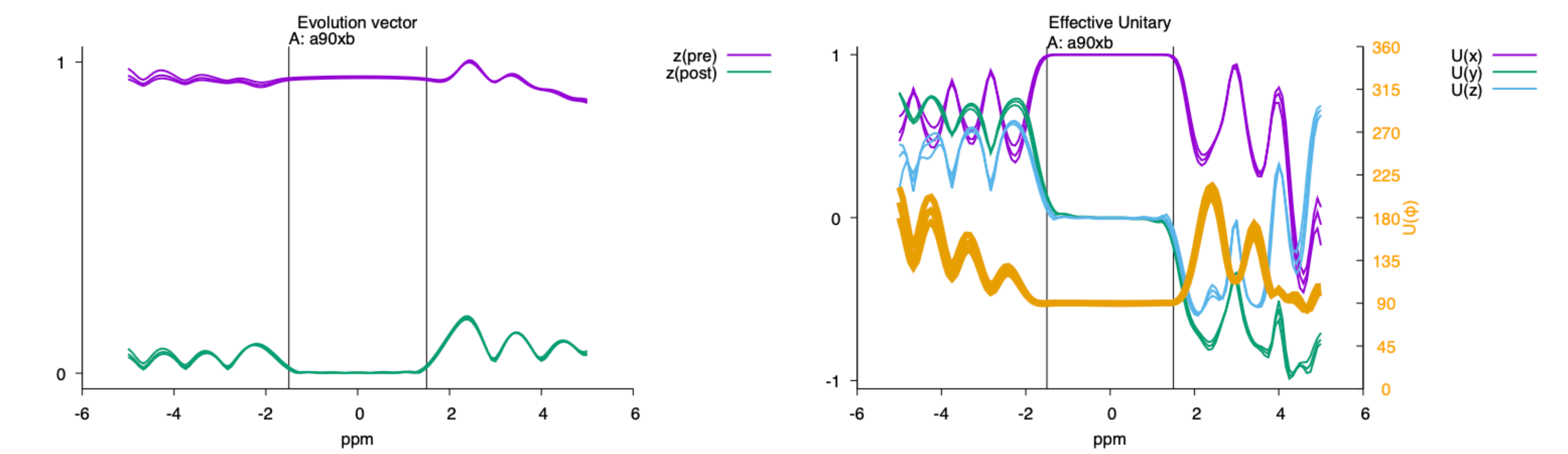
The first plot shows the “pre” evolution delay inside the optimised band is the required 0.95 of the total
duration. The “post” evolution delay, as required is zero. The second plot shows the central zero-time
rotation versus frequency. During the optimised band the pulse is doing a perfect 90x. Outside of the
optimised band, performance is uncontrolled.
When analysing 180∘ pulses, use the HALF flag. The analysis splits the pulse into two, and shows the pre,
post and central evolution periods, and the central-zero-time unitary rotation of the front and back halves.
For a good refocusing 180∘ pulse you want the middle delay to be zero, and the central unitaries to be 90∘
rotations around the same axis.
Seedless can optimise pulses whose amplitudes or phases are represented by a series, similar to the original BURP pulses. This feature was added following requests from Alex Hansen. In our tests, phase-only GRAPE pulses usually outperform these lower-dimensional series descriptions, but the option is useful for exploring smooth pulse forms and for comparison with traditional shaped pulses.
For a Fourier representation, the phase can be written as:
| (3) |
To use this mode, define the number of parameters to optimise in the Fourier series. For F Fourier terms, the number of parameters is P = 2F + 1:
SERIES FOURIER 5
Assuming no transient response, the derivatives are:
| (4) |
where Pj is the relevant Fourier coefficient. With k numbered from 0 to N − 1:
| (5) |
Seedless already contains the values of 2Tr(BiCk), so the implementation pre-computes the derivative factors and adds a loop over the Fourier coefficients.
Two useful modifiers are available. If amplitudes are being optimised, SERIES_ZEROEDGES forces the pulse
amplitude to start and end at zero by constraining a0 to be related to the other constants ak. This
removes one parameter from the fit. The command FOURIER_COSONLY ignores all sine coefficients,
bj.
A power-series representation is also available, although there is no obvious physical reason to prefer it. The expansion is taken about the centre of the pulse:
| (6) |
It is enabled with:
SERIES POWER 10
The number specifies the number of parameters. As for the Fourier series, SERIES_ZEROEDGES can
be used during amplitude optimisation to force the pulse to start and finish at zero. In tests,
power-series pulses are close to, but slightly worse than, Fourier-series pulses with a similar number of
parameters.
Overall, the results from series optimisation are not especially encouraging. Phase-only constant-amplitude pulses generally give better fidelity, often by an order of magnitude or more. Series optimisation can also be tricky, and horserace mode may be needed to find a reasonable minimum. Smooth series pulses may still be useful on hardware with a limiting response function, but for most Seedless applications, allowing the optimiser to control all finite elements directly is more effective. In the demo, there is an example where we compute a pulse that looks identical to the EBURP from scratch using this mode.
The command HESSIANPLOT adds Hessian characterisation to the report. Seedless computes a numerical
Hessian matrix from central differences of gradients:
| (7) |
where gi(x) is the gradient with respect to parameter i at parameter vector x. The eigenvalues of the real symmetric hessian are then computed and ranked. If all eigenvalues are positive, the point is a true local minimum. If the eigenvalues contain a mixture of positive and negative values, the solution is a saddle point.
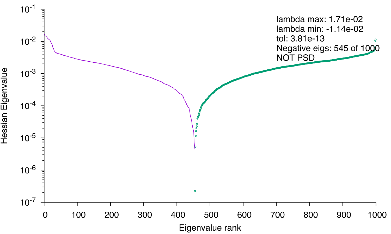
The following example is a phase-only pulse designed to perform a band-selective state-to-state transformation Iz →−Iy while preserving Iz → Iz outside the band, similar to an EBURP1. For random initial phases, the hessian contains a mixture of positive and negative eigenvalues:
After optimisation with near-default settings, 𝜖 = 10−10, the pulse converges in about 40,000 steps:
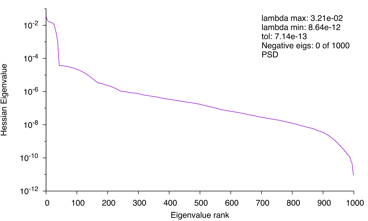
Driving the optimisation harder, using 𝜖 = 10−14, gives convergence in about 200,000 steps:
The final Hessian is positive definite. This analysis can therefore distinguish a true minimum from a saddle point. In this example, the difference in pulse shape and infidelity between the last two cases is tiny.
For phase-only optimisation, Seedless usually gets close to, or reaches, a true minimum. There are exceptions, especially for difficult problems where a small probability of a local minimum remains; horserace mode is useful in those cases. For amplitude and phase optimisation, the solutions often appear to be saddle points. This fits the intuition that the optimiser has multiple similar descent directions involving changes in either amplitude or phase. We therefore recommend phase-only optimisation, followed by conversion to an amplitude/phase pulse only if reduced integrated B1 is genuinely required. In practice, it does not seem to matter whether the solution is a true minimum or a saddle point, provided the cost function (infidelity) is sufficiently small.
As part of the phase-only pulse work, Seedless includes two conversion modes that explore the equivalence between phase-only and amplitude/phase pulses. These may be useful when integrated B1 power must be minimised.
Add AMPtoPHASE to the header to create an additional phase-only version of an amplitude-modulated
pulse. This works well with Make mode for traditional pulses such as EBURP, REBURP, and CHIRP.
Seedless uses a Trotter–Suzuki mapping that increases the number of finite elements by a factor of 4,
following the practical pulse-engineering approach used to avoid unnecessary matrix exponentiation.[?]
Each new element uses the maximum supplied amplitude, while preserving the same total pulse
duration.
The infidelities of the original amplitude/phase pulse and the converted phase-only pulse are usually similar. If desired, the converted pulse can be read back into Seedless for further optimisation.
The reverse conversion is less direct. When reading in a phase-only pulse, specify PHASEtoAMP, optionally
followed by an integer smoothing window. Seedless computes the complex value associated with each finite
element, ω1eiϕi, and applies binomial smoothing. The smoothing window should be odd. A value of 5 gives
weights proportional to 1:4:6:4:1.
After conversion, the pulse is read in and a phase-only optimisation is performed with fixed amplitudes. This can reduce the amplitude requirement. The process can be repeated until the B1 requirement is reduced without significantly compromising infidelity.
For routine NMR work, we have generally not needed to reduce B1: running at maximum field for a few milliseconds is usually acceptable on modern hardware. In other fields, such as MRI, this may be less true. These conversion modes provide a compromise when lower integrated power is important.
The original Seedless implementation used liblBFGS from Naoaki Okazaki (link), a faithful C++
implementation based on the original LBFGS algorithm by Jorge Nocedal. LBFGS, BFGS, SR1, and Newton
methods are all related quasi-Newton or Newton-type optimisers that use, approximate, or build information
about the hessian.
We highly recommend the default but the other optimisers can be selected with:
optimiser liblBFGS # default
optimiser lBFGS
optimiser BFGS
optimiser Newton
optimiser SR1
optimiser Hybrid 15
| Optimiser | Comment | Recommendation |
| liblBFGS | Default implementation. Fast and robust in tests. | Use for normal work. |
| lBFGS | Alternative LBFGS implementation. | Available for comparison. |
| BFGS | Builds a fuller hessian approximation. | Usually slower and less useful here. |
| SR1 | Alternative quasi-Newton update. | Usually slower and less useful here. |
| Newton | Uses analytical hessians. Can reduce iteration count. | Each function call is much more expensive. |
| Hybrid 15 | Runs the specified number of Newton iterations, then switches to lBFGS. | Experimental. |
In our tests, there is usually no reason to use anything other than liblBFGS. BFGS and SR1 tend to take
longer and are less able to find good minima. Newton’s method can descend rapidly for favourable initial
seeds and may find a good pulse in roughly 10 fewer iterations, but each function call can be more than 100
times slower. Overall, liblBFGS and Newton find similar minima, with liblBFGS being much faster in
wall-clock time.
All these methods also require a line search. The optimiser defines a search direction, but a separate
decision is needed about how far to move in that direction. Different implementations handle this step
differently, and this can affect performance. In our testing, it is hard to beat the behaviour of liblBFGS and
the original lBFGS line-search strategy.
This section serves as a reference for editing Seedless input files. It is deliberately more detailed than the introductory examples and is intended for consultation rather than sequential reading. Use it when you want to modify the behaviour of a calculation, add restraints, change the output format, or simulate an existing pulse.
Note
Seedless input files have two main parts. The first part is the header, which contains one-line commands such as frq, pulseName, Bruker, and maxIter. The second part contains named sections, such as RF:, Plot:, SpinSystem:, Carriers:, wmH:, Durations:, and Targets:. Once Seedless reaches one of these named sections, it stops reading header commands.
A typical input file has this overall structure:
# Header commands first
frq 150
pulseName my_pulse
Bruker
MakeSummary
# Then named sections
RF:
  1.0 1.0
Plot:
  P 0 200 120
SpinSystem:
  CO 165 185 96
Carriers:
  176
wmH:
  17605
Durations:
  130E-6 130
Targets:
  Iz -Iz
Header commands control the global behaviour of the calculation: where output files go, how pulses are named, whether Bruker, Varian or Jeol pulse files are written, how much optimisation is performed, and which optional analysis modes are switched on.
| Keyword | Default | Purpose |
| frq | 150 | Larmor frequency of the nucleus, in MHz. |
| outPath | ./ | Directory where output files are written. |
| pulseName | auto | Sets the output pulse name. If omitted, Seedless builds a name from the restraints, carrier, field, duration, and miss weights. If set, pulses are named name_A, where A is an integer starting from 1. |
| MakeSummary | false | Generates the formatted PDF summary report. Requires gnuplot and pdflatex. |
| DATETIME | false | Add a date/time stamp to the report. Requires the LaTeX datetime package. |
| seed | 123 | Random-number seed used to initialise the calculation. |
| CalcInit | false | Include the initial state in the final report. |
| LINK | false | Link the target list with the duration/point list so that corresponding rows are used together rather than forming an independent grid. |
| Keyword | Default | Purpose |
| Bruker | false | Uses Bruker conventions for reading and writing pulse files. This reverses the direction of Y evolution in outputs/read-in pulses, sets writeBruker, and adjusts the default read-in columns for Bruker files. |
| writeBruker | false | Write Bruker-format pulse output. |
| writeVarian | false | Write Varian-format pulse output. |
| writeJeol | false | Write Jeol-format pulse output. |
| GNUEPS | false | Write gnuplot figures as EPS rather than PDF. |
| GNUPNG | false | Write gnuplot figures as PNG rather than PDF. |
Seedless can read and write both Bruker and Varian-style pulse files. The differences are primarily formatting conventions, although there is also an important difference in phase convention. If you are working on a Bruker spectrometer, include the following keyword in the header:
Bruker
This switches Seedless to Bruker conventions for both reading and writing pulses (do not use this if you want
Varian and Jeol pulses!). It also sets the Bruker read-in defaults automatically. Use MakeSummary if you want
the report plots, and use Bruker shapetool to check how the pulse will be perceived by the
spectrometer. If the Seedless report and shapetool disagree, treat shapetool as the hardware-facing
reference.
| Format | Column order | Amplitude scale | Seedless settings |
| Bruker | amplitude, phase | 0–100 | ReadColAmp 1, ReadColPhi 2, ReadMaxAmp 100 |
| Varian | phase, amplitude | 0–1023 | ReadColPhi 1, ReadColAmp 2, ReadMaxAmp 1023 |
| Jeol | n, phase, amplitude ,n | 0–100 | ReadColPhi 2, ReadColAmp 3, ReadMaxAmp 100 |
For example, a Bruker-style file has amplitude first and phase second:
100, 0
100, 180
100, 0
100, 180
...
A Varian-style file has phase first and amplitude second:
0,   1023
180, 1023
0,   1023
80,  1023
...
A Jeol-style file has phase second and amplitude third (we do not use the 1st and 4th columns):
1, 0,   100, 0
1, 180, 100, 0
1, 0,   100, 0
1, 180, 100, 0
...
Varian-style input is the default, by virtue of Lewis Kay’s NMR centre being Varian until relatively
recently. To write a pulse for direct use on a spectrometer, specify writeVarian, writeBruker or writeJeol.
The Bruker keyword sets Bruker read/write conventions and reverses the relevant phase convention for
read-in and written pulses.
Seedless uses the following RF Hamiltonian internally, which is also the Varian and Jeol convention:
| (8) |
The Bruker convention is effectively:
| (9) |
Here ω is the applied B1 field in radians per second, and Ix and Iy have their standard meanings.
Seedless always performs its internal calculations using Equation 8. When Bruker is set, phases are
inverted at read-in and write-out so that Seedless, Bruker hardware, and shapetool behave
consistently.
This convention affects the relative sense of rotation in the xy plane compared with intrinsic spin evolution such as chemical shift and J coupling. In experiments such as TROSY, getting these relative signs correct can be crucial. If a sequence does not behave as expected, useful tests are to reverse the target rotation direction and/or add 180∘ phase-cycle changes at the relevant points in the pulse sequence.
The default optimiser settings should be reliable. Increase ncpus to make use of all available processor cores. For final polishing, setting maxIter to a larger number ensures the optimisation continues until convergence.
| Keyword | Default | Purpose |
| ncpus | 1 | Number of processors used to share the work. |
| maxIter | 1000 | Maximum number of iterations for the main optimisation. A value of 0 disables the iteration limit and allows optimisation to continue until convergence. |
| NoOpt | false | Simulate/report the pulse without running the optimisation. |
| OptAmp | false | Optimise amplitudes as well as phases. |
| NoOptPha | false | Do not optimise phases. This is typically used only for specialised amplitude-optimisation tests. |
These settings control the optimiser used for both the main optimisation and, where relevant, the horserace stage. The default optimiser is libLBFGS, which is recommended. For more information on these see the liblBFGS documentation.
| Keyword | Default | Purpose |
| gtol | 0.5 | Controls the accuracy of the line search routine. |
| epsilon | 10−10 | Inter-interation convergence test. |
| hessianM | 300 | The number of corrections to approximate the inverse hessian matrix. |
The optimiser is selected with one of the following lines:
optimiser liblBFGS
optimiser Newton
optimiser BFGS
optimiser SR1
optimiser lBFGS
optimiser Hybrid 15
optimiser Hybrid 15 runs 15 iterations of Newton–Raphson optimisation, followed by lBFGS. In our tests, libLBFGS and lBFGS significantly out-perform all the other optimisers. But they are there if you want to play with them. Analytical Hessians are efficiently computed when using the Newton–Raphson scheme.
| Keyword | Default | Purpose |
| iterPrint | 0 | Generates an intermediate PDF report every specified number of iterations. The default writes only the final report. |
| iterShow | 1 | Print status to the screen every specified number of iterations. |
| iterShowFac | 2 | Increase the printing interval by this factor. Use 1 for a linear interval. |
| Keyword | Default | Purpose |
| initPha | rand | Initialise phases randomly, or set to zero |
| initAmp | 1 | Initialise phases at one, or set to rand |
| IterAmpM | 0.5 | Initial random amplitudes will be initAmpM*rand+initAmpC where rand is between 0 and 1. |
| IterAmpC | 0.0 |
|
| ampWeight | 1 | Decrease to emphasise amplitudes and vice versa in phase/amp optimisation. |
| alpha | 1 | Apply an amplitude penalty if normalised amplitudes exceed 1. |
| alphaS | 10−12 | Apply a smoothing penalty on the amplitudes. |
| smooth | 0 | Apply a moving average to phases over this number of points. |
Formal symmetries can be imposed on the pulse phases. These can help in some cases, but they can also make a pulse worse if the best solution does not have the imposed symmetry.
| Keyword | Default | Purpose |
| SYM | false | Impose time-reversal symmetry on the pulse phases. This gives a symmetric frequency response. |
| SYMPR | false | Impose time reversal plus phase inversion. |
| WritePR | false | Write a time-reversed, phase-flipped pulse in addition to the normal output. |
| AMPtoPHASE | false | Convert an amp/phase pulse to a phase-only pulse; see Section x1-550009.89.8. |
| PHASEotAMP | 5 | On read in, create an amplitude/phase modulated pulse from a phase-only; see Section x1-550009.89.8 |
Broadband inversion pulses (BIPs) often benefit from SYM. If the best solution has a symmetry, the optimiser finds it naturally. If imposing symmetry gives worse performance, remove the symmetry constraint.
The horserace tests several random seeds for a short optimisation and then continues with the best one. This is useful when the optimisation is sensitive to the initial random phases; see Section x1-480009.19.1.
| Keyword | Default | Purpose |
| Horsey | 50 | Run a horserace using this number of random seeds. An integer is added to seed for each trial. The best seed is saved and used for the full optimisation. |
| HorseyIter | 100 | Number of iterations allowed for each horserace trajectory. |
| HorseyBins | 10 | Number of bins used in the final horserace histogram. |
Grid search lets you scan over pulse parameters such as field strength, total duration, or finite-element duration. This mode runs the grid search and then quits; it does not currently run a horserace or random-seed testing as part of the same calculation.
| Command form | Example | Purpose |
| Grid Iter | Grid Iter 1000 | Turn on grid search and set the maximum iterations for each grid point. |
| Grid Show | Grid Show 5 | Show sampled grid-search trajectories every specified number of iterations. |
| Grid X list | Grid B1 list 5000 7500 10000 | Uses the explicitly listed values for X. Here X can be B1, T, or dt. |
| Grid X A B C | Grid T 5 100E-6 200E-6 | Construct a linear series with A values from B to C. Here X can be B1, T, or dt. |
For each frequency, Seedless can analyse a pulse as a pre-evolution delay, a central zero-time unitary rotation, and a post-evolution delay.[?] This is the analysis mode used for the evolution-controlled pulses created with the targets discussed in Section x1-520009.59.5. A good evolution-controlled pulse should have these factors roughly constant across the chemical-shift range.
| Keyword | Default | Purpose |
| EVOLVE | false | Perform the schematic pulse analysis. |
| HALF | false | Perform the schematic pulse analysis at the halfway point. This is important for 180∘ refocusing pulses. |
| REBURP | false | Apply a90xb at the halfway point of unitary bands. |
| evAlpha | 0.0 | Sets a when creating a90xb targets. |
| evBeta | 0.0 | Sets b when creating a90xb targets. |
Use HALF when analysing 180∘ refocusing pulses. The Euler description has a gimbal-locking singularity for 180∘ pulses, and analysing the pulse halfway through avoids this problem.
Use Read to read in an existing pulse. This is most often used with NoOpt, so that Seedless simulates the pulse without changing it. If NoOpt is omitted, Seedless will use the read-in pulse as the initial condition for optimisation; this often gives a local minimum, and starting from random phases is usually better.
Before reading a pulse, make sure the amplitude and phase columns are specified correctly. If Bruker is set in the header, the Bruker read-in defaults are set automatically. Otherwise, Seedless defaults to Varian-style input.
| Keyword | Default | Purpose |
| ReadMaxAmp | 1023 | Maximum amplitude value in the file. This corresponds to the maximum B1 field. Use 100 for Bruker and Jeol, and 1023 for Varian unless your file uses a different convention. |
| ReadColAmp | 2 | Column number containing amplitudes. Default is 1 for Bruker and 2 for Varian and 3 for Jeol. |
| ReadColPhi | 1 | Column number containing phases. Default is 2 for Bruker and Jeol, and 1 for Varian. |
The simplest Read command is
Read Gaus1.1000
Options can be added on the same line:
| Option | Effect |
| phase A | Add A degrees to all phases. |
| rev | Reverse the time elements and flip the phase. |
| duration A | Set the total pulse duration to A. In this context, use seconds, as in 2E-3. |
| field A | Set the peak B1 field to A Hz. |
| pre A | Add a pre-delay of A seconds. |
| post A | Add a post-delay of A seconds. |
| concatenate A | Repeat the element A times. |
For example, this reads Hello.RF, sets the total duration to 2 ms, and simulates it at a peak B1 field of 20 kHz:
Read Hello.RF duration 2000 field 20000
Special pulse names are also available. Free inserts a period of free precession for the specified duration. A name of the form HardXXX creates a rectangular pulse with a flip angle of XXX degrees on resonance. You can concatenate as many Read lines as needed.
To convert a phase-only pulse into an amplitude/phase approximation, use:
PHASEtoAMP 5
This applies binomial smoothing. It is useful when you want to approximate a phase-only pulse by an amplitude/phase pulse and then reoptimise. Repeated cycles often give similar infidelity while reducing the integrated B1 requirement.
Seedless can create Q3, Q5, SEDUCE, REBURP1, EBURP1, BURP1, HARD, and adiabatic pulses such as CHIRP, TANH, CHORUS, and WURST. A pulse file can also be supplied ,and the following B1 optimisation will be performed on an arbitrary waveform.
A simple example is:
Make Q5 1000 1000 Opt Iz Iy -1
This creates a Q5 pulse with 1000 elements and a total duration of 1 ms. In Make commands, the duration is given in μs. The Opt Iz Iy -1 part asks Seedless to optimise the field so that, on resonance, the pulse transfers Iz to −Iy. After making a pulse, Seedless produces the report and quits, so Make overrides other calculation instructions.
You can also read in a pulse, fix its duration, and determine the optimal on-resonance field. For example:
Make make/pulse_Q5_1.RF 1000 1000 Opt Iz Iy -1
This reads a Q5 pulse of duration 1 ms and finds the B1 field required for a 90∘ rotation, which is 4546 Hz in this example. If the input file uses Bruker format, put Bruker in the header so that ReadColPhi, ReadColAmp, and ReadMaxAmp are set correctly.
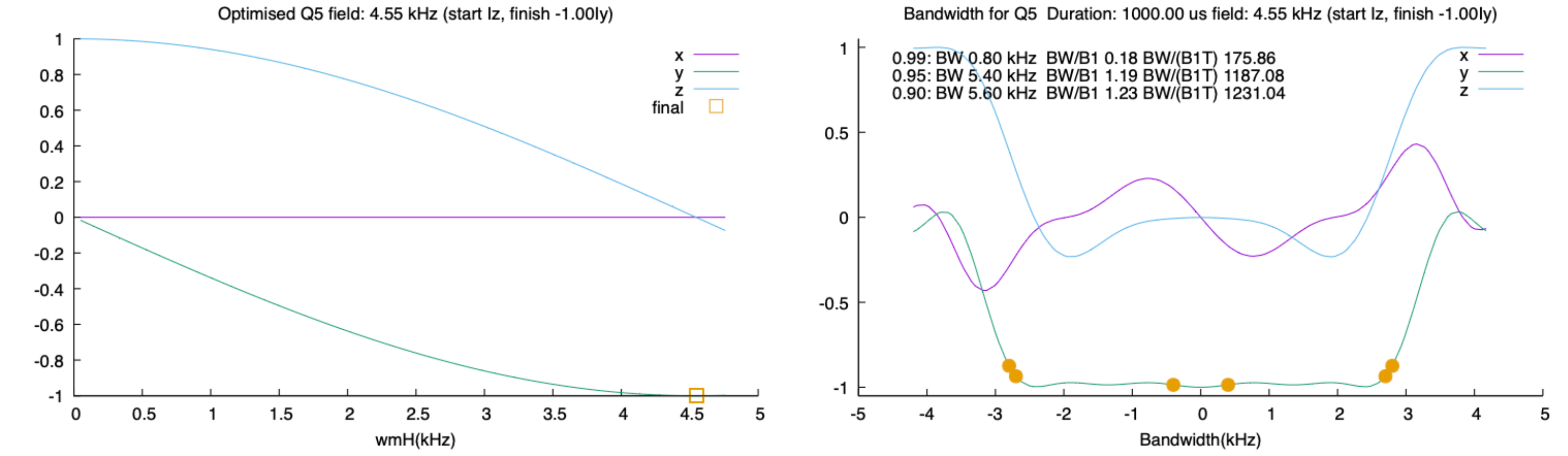 The first plot follows pulse performance versus B1 and runs a simple optimiser to find the field with
peak performance. The second estimates the 0.99, 0.95, and 0.90 points of the excitation window. This is
convenient for quick calibration of standard pulses.
The first plot follows pulse performance versus B1 and runs a simple optimiser to find the field with
peak performance. The second estimates the 0.99, 0.95, and 0.90 points of the excitation window. This is
convenient for quick calibration of standard pulses.
Additional Make options include:
| Option | Effect |
| NoFitBandwidth | Skip the bandwidth analysis. Use this if the calculation hangs during bandwidth fitting. |
| Profile A B v | Profile only; do not optimise B1. Start from A, finish on B, and use sign/value v. |
| Opt A B v | Optimise B1. Start from A, finish on B, and use sign/value v. |
| wHmax | Set the maximum B1 value used in the profile. |
| SetB1 | Manually set the peak B1. |
| offset | Apply a phase ramp to the pulse by frequency. |
| shift | Synchronise the phase ramp with the pulse end. |
| rev | Time-reverse the pulse. |
| offmax | Set the maximum offset used in the profile. |
| tag | Add a string tag to the pulse name. |
| phase | Add phase; use values 0, 1, 2, or 3. |
For an adiabatic example:
Make CHIRP 1000 2000 sweep 20000 n 5 SetB1 4060 Opt Iz Iz -1 wHmax 10000
Here, sweep sets the frequency-sweep width and n sets the amplitude-profile shape. Additional adiabatic options are:
| Option | Effect |
| sweep | Set the adiabatic sweep width. |
| kappa | Set the sweep rate in MHz s−1 for TANH and WURST pulses. |
| n | Set the amplitude-profile shape for CHIRP, WURST, TANH, and CHORUS. |
| ADIABATIC | Analyse how adiabatic the pulse is. |
The calibrate demo project contains useful examples. Remove the initial # in that demo file to execute a line . Note if you have multiple Make lines, Seedless will treat this literally and concatenate multiple pulses. This probably isn’t what you want.
Make Q5 1000 1000 Opt Iz Iy -1
Make Q3 1000 1000 Opt Iz Iz -1
Make SEDUCE 1000 1000 Opt Iz Iz -1
Make REBURP1 1000 1000 Opt Iz Iz -1
Make EBURP1 1000 1000 Opt Iz Iy -1
Make HARD 1000 500 Opt Iz Iy -1
Make CHIRP 1000 2000 phase 2 sweep 20000 n 5 SetB1 4060 Opt Iz Iz -1 wHmax 10000
Make CHIRP 1000 2000 sweep 20000 n 5 SetB1 1060 Opt Iz Iy -1
Make TANH 1000 2000 sweep 20000 kappa 0.005 n 5 SetB1 1060 Opt Iz Iz -1 wHmax 5000
Make CHORUS 2000 2000 sweep 300000 n 5 SetB1 15500 Profile Iz Ix 1 wHmax 20000
As described in Section x1-530009.69.6, amplitudes and/or phases can be represented by either a Fourier series or a power series.
SERIES FOURIER 5
SERIES POWER 10
FOURIER_COSONLY
SERIES_ZEROEDGES
Do not specify both series types in the same calculation. Fourier/power-series modes are useful for reproducing some older BURP-style computations[?], but for most modern Seedless calculations a phase-only pulse is usually more effective.
As described in section 9.7 for diagnostic calculations, use:
HESSIANPLOT
TESTGRADS
HESSIANPLOT computes the Hessian and its eigenvalues for the final report; see Section x1-540009.79.7. TESTGRADS compares analytical and numerical gradients and reports the absolute gradients at the point where the calculation stops.
Named sections come after the header. They can appear in any order, and each section can contain as many lines as needed. Once Seedless reaches a named section, it no longer treats subsequent lines as header commands.
Use RF: to describe the B1 homogeneity distribution. Always include this section. If you do not want B1 compensation, include a single line with 1.0 1.0.
| Column | Example | Meaning |
| B1 | 0.93 | Relative B1 field. 1.0 means the calibrated peak field. |
| weight | 0.25 | Relative weight of this B1 value in the optimisation. |
RF: (B1/weight)   # one row per B1 homogeneity value
0.93 0.25
1.00 0.50
1.05 0.25
Use Plot: to choose the offsets shown in the final report. The plotting grid should not exactly match the optimisation grid in SpinSystem:; otherwise you only see performance at the points used during optimisation. Always include this section, even if you use only a small number of plotting points.
Plot: (Min/Max/Num)  # for showing final profiles
P 0 200 120
You can also apply different relative B1 values in different ppm ranges:
Plot: (Min/Max/Num)
P 0 5 60 B1 0.5
P 5 14 60 B1 1.0
List ppm ranges from low to high so that output plots are continuous.
Use SpinSystem: to specify the chemical-shift bands included in the optimisation. The first entry is an arbitrary band name. For a simple pulse with one chemical-shift range, use one line. For selective pulses with several bands, use one line per band.
| Name | Min ppm | Max ppm | Num | Meaning |
| CO | 165 | 185 | 96 | Optimise over 96 CO offsets from 165 to 185 ppm. |
SpinSystem: (Min/Max/Num) # one row per group of spins
CO 165 185 96
CA 40 78 96
CB 8 40 96
Use Carriers: to specify the carrier frequency, in ppm. This is the centre of the pulse.
Carriers: (ppm)
176
Use wmH: to specify the calibrated peak B1 field in Hz. This value is important: it should be measured for your probe, sample, and amplifier settings.
For a direct-dimension calibration, measure a nutation curve. If the 360∘ rotation time is t360, the corresponding B1 field in Hz is 1∕t360. For example, a 14.2 μs 90∘ pulse corresponds to a field of 17605 Hz. For a heteronucleus, a practical approach is to use an HSQC-based calibration in which a test pulse is inserted after the first INEPT on the insensitive spin.
For low-γ nuclei, the field generated by the amplifier is often relatively sample independent. This is less true for protons. For maximum sensitivity, calibrate the relevant B1 values and use those values in the Seedless calculation.
wmH: (Hz)
17605 # 14.2 us 90-degree pulse time
Use Durations: to specify the total pulse duration and the number of finite elements. If you want duration rows to correspond one-to-one with target rows, rather than forming an independent grid, use LINK in the header.
| Column | Example | Meaning |
| Total | 130E-6 | Total pulse duration, in seconds. |
| points | 130 | Number of finite elements. |
Durations:
130E-6 130
Use Targets: to start the section showing which transformation the pulse should perform. You can provide as many target rows as needed. Each row must contain one target instruction for each chemical-shift band in SpinSystem:. Separate band instructions with commas and leave spaces around the commas. Targets should be provided in the same order as the bands.
Some common examples for excitation (taking the spin from longitudinal, moving into the XY plane. Difficulty (and hence relative pulse duration) increases down the table. EV indicates evolution control[?].
| Type | Example | When you would use |
| XYcite | Iz Iex | Take longitudinal magnetisation into the XY plane as rapidly as possible. |
| State-to-state | Iz -Iy | This is an excitation, use to start/finish INEPT transfers and indirect evolution elements. |
| State-to-state EV | Iz -0.5OIy | A state-to-state excitation with a controlled ‘post’ evolution period. |
| Universal | 90x | Create a pulse that performs like a true 90o rotation about the x axis |
| Universal EV | a90xb | Create a pulse that performs like a true 90o rotation about the x axis, with pre and post evolution delays set by evAlpha and evBeta |
For 180o rotations,
| Type | Example | When you would use |
| State-to-state | Iz -Iz | An inversion, used in decoupling / INEPT transfers |
| Universal | 180x | For refocusing, a 180o rotation about the x axis. |
| Universal EV | 180x+ REBURP | For refocusing, a 180o rotation about the x axis with evolution control, specified by evAlpha and evBeta |
You are free to mix and match state-to-state and universal restraints for different bands.
For state-to-state targets, give the starting state and final state separated by a space. Choices for states are Iz, Iy, Ix, -Iz, -Iy, -Ix and Iex. State-to-state restraints can also be supplied as a single string (no spaces) as linear combinations, for example 0.5Ix+0.5Iy. For a problem with three bands the targets should look like this
Targets:
Iz -Iz , Iz Iz , Iz Iz
For universal targets, give a single operator such as id for an identity restraint (the state at the end has to
exactly match the state at the beginning), 90x (90o rotation about the x axis), 180x (180o rotation about the
x axis) or a90xb (90o flanked by fractional pre and post evolution periods specified by evAlpha and evBeta
in the header), for example
Targets:
90x , id , id
A more general syntax is available for universal restraints. The unitary operators have the form e−iA, where

Here, B sets the flip angle, P sets the phase in units of π, and O sets evolution about Z for a fraction of the total duration for evolution control. For example, 0.25B is a 90x restraint, and 0.35B+0.5P is a 126y-type restraint. Multiple propagators can be concatenated with semicolons:
0.25B+0.5P;0.5B;0.25B+0.5P
This creates a 90y pulse, followed by a 180x pulse, followed by another 90y pulse, and
0.3O;0.25B;0.6O
This creates a schematic pulse with a ‘pre’ delay of 0.3 times the pulse length, and a ‘post’ evolution delay
equal to 0.6 times the pulse length, flanking a 90x central rotation. This is equivalent to specifying a90xb,
and setting evAlpha 0.3 and evBeta 0.6.
The XYcite restraint was modified, with thanks to Jesse Shelfhout, to support laser-excitation work. The original XYcite pulse selected for “not Z”. The command
XYciteTarg 0.707
can be set in the header to set the desired amount of Z remaining in the final state. If this value is omitted or set to zero, Seedless selects for “not Z”. If it is set to 1.0, the pulse tries to end with only Z. A value of 0.707 gives approximately equal excitation and remaining Z magnetisation. This is useful when transverse relaxation is fast and only a small fraction of the total magnetisation should be tipped into the transverse plane, allowing a faster repetition delay.
This determines the angle 𝜃 of the final magnetisation relative to the Z axis, with XYciteTarg = sin(𝜃). Different bands can be used to specify specific XYcite target excitation values. For example:
Targets:
Iz 0.5Iex ,  Iz 0.1Iex , Iz 0.2Iex ....
sets different excitation amounts for each band.
A state-to-state evolution-controlled target can be created using syntax such as:
Targets:
Iz -0.5OIy
The capital letter O before Iy triggers this mode, and note that the minus sign applies to the Iy rather than
to the 0.5. The target starts from Iz and ends at the appropriate point in the transverse plane, taking into
account the chemical shift of the spin and half of the pulse length. In the ‘schematic picture’ this will create a
pulse with uncontrolled ‘pre’ evolution, and have a controlled ‘post’ evolution equal to half of the pulse
duration[?].
This mode can also use XYciteTarg when small flip-angle excitation is desired. If 𝜃 is the angle
to the z axis and XYciteTarg is sin(𝜃), then the target -0.5OIy creates the reduced density
matrix:
| (10) |
In this expression, XYciteTarg sets the angle to the z axis, while the offset-dependent command rotates the
final transverse state by the desired amount of chemical-shift evolution. This syntax can therefore be used to
make small-flip-angle, state-to-state, evolution-controlled pulses.
In terms of difficulty, a fully evolution-controlled unitary pulse is usually the most demanding. A unitary 90∘ pulse is typically easier because it does not control evolution. A state-to-state evolution-controlled pulse is probably comparable in difficulty to a normal state-to-state pulse, and XYcite is easier again.
Use BandWeight: to change the relative applied B1 weighting in different bands. Each line must contain one entry per band, matching the order used in Targets:. Add multiple lines to test multiple combinations.
For example, with two bands, this applies 50% of the maximum relative B1 to the first band and 100% to the second:
BandWeight:
0.5 , 1.0
Use Miss: to add a miss restraint, commonly used for water suppression or for protecting a region while optimising another region.
| Name | Min ppm | Max ppm | Num | Target and options |
| Wat | 4.65 | 4.85 | 10 | Apply the following target over 10 linearly spaced ppm values. |
Miss: (Min/Max/Num/Target) # one row per group of spins
Wat 4.65 4.85 10 Iz Iz stride 2 weight 1
This applies the Iz Iz start/finish restraint to 10 ppm values spaced linearly between 4.65 and 4.85 ppm. stride controls how often the restraint is applied: stride 1 means every finite element, stride 2 means every other element, and so on. weight controls the relative importance of the miss restraint. Increase it if the calculation should pay more attention to this region. We are very grateful to Steffen Glaser for helping revise how we compute the miss restraint (section 10.4.9)
The derivation below is retained for readers who want the implementation detail behind the miss-restraint speedup. It is not needed for routine pulse design.
Following discussion with Prof. Steffen Glaser, it was pointed out that our water-miss pulses are identical in formulation to previously published optimal-tracking pulses. The original Seedless implementation evaluated gradients using a triangular sum. For a cost function with N finite elements, where the effect of the pulse is recorded at every element, the original expression was:

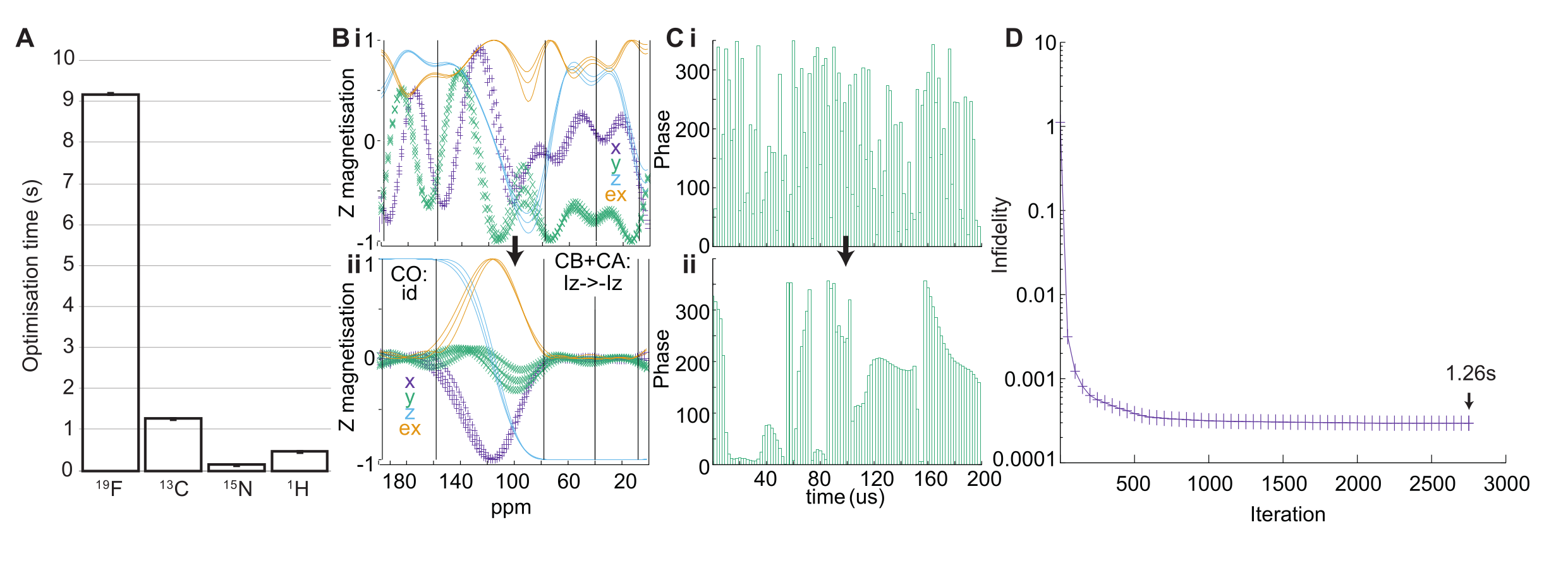
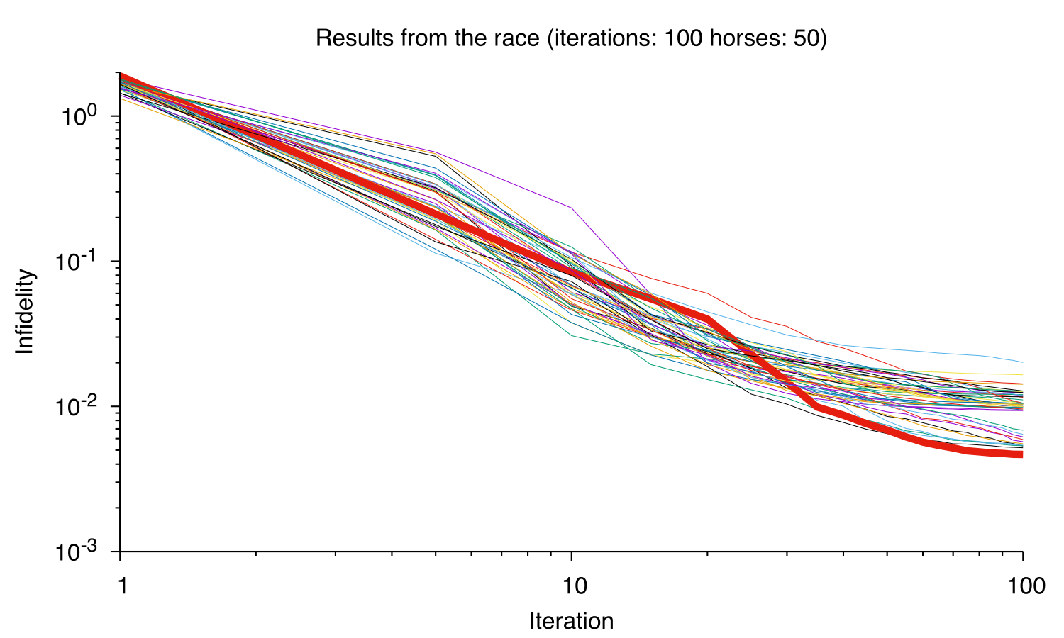
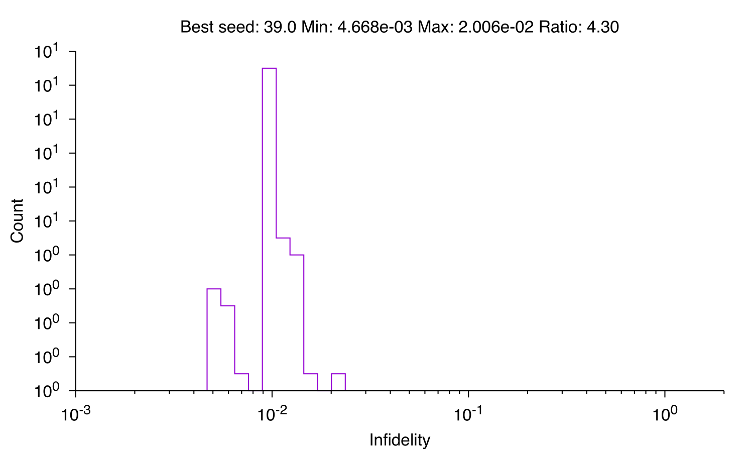
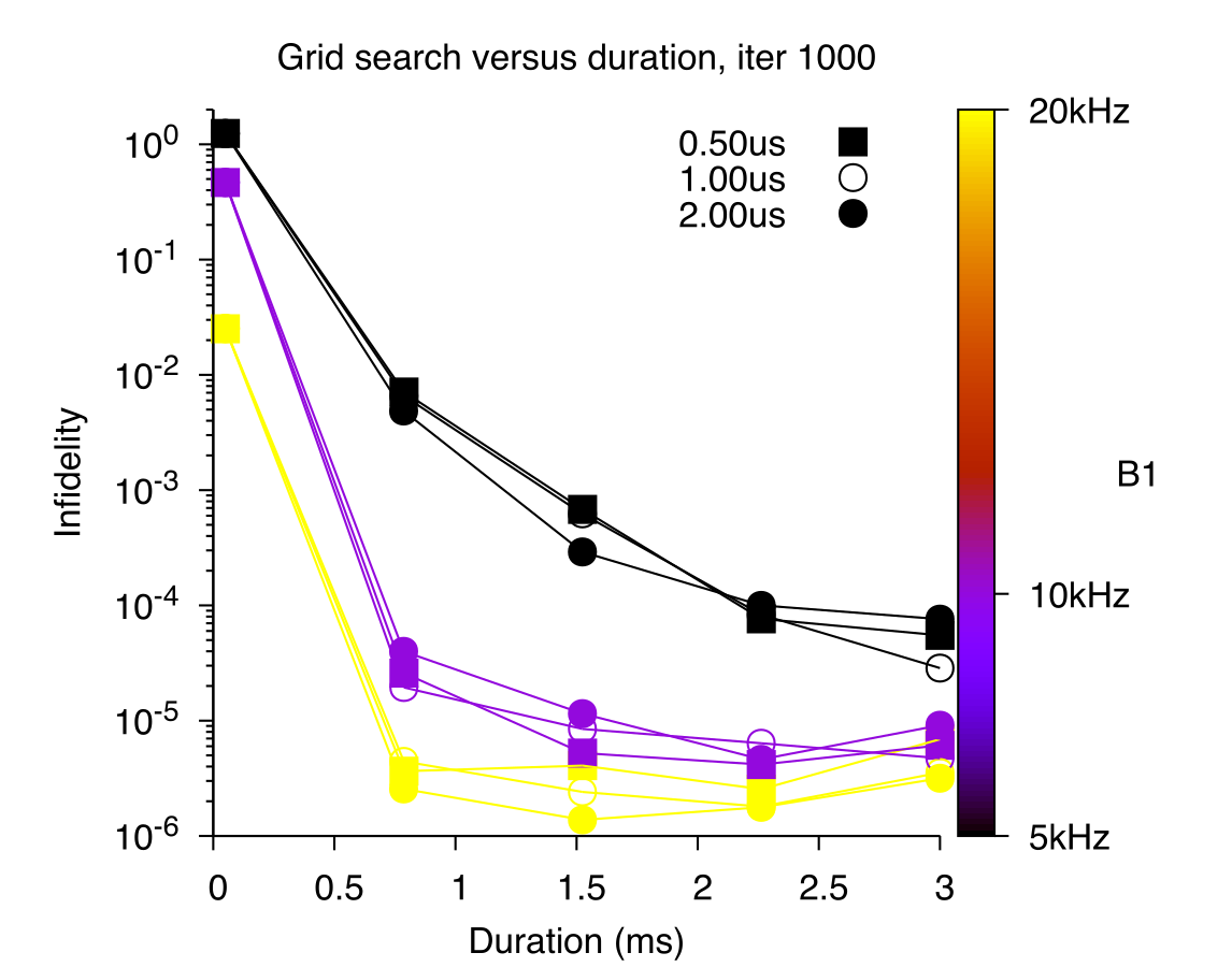
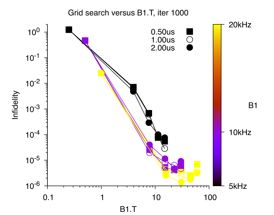
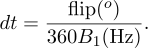
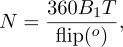

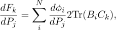
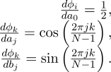
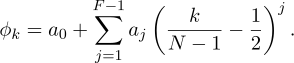





 Tr
Tr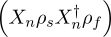
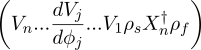



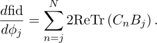
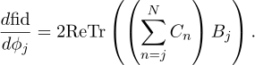
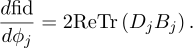
 pulses
 nuclei when quadrupolar interactions have averaged to zero. If you have strong
coupling, or you have the pulse on multiple nuclei at once, then make the pulse short. These ideas lead to the
“schematic pulse” description of pulses, and “evolution controlled” pulses that exactly control both scalar
coupling and chemical shift evolution times in pulse sequences. These ideas are described in a paper with by
S. Lim, B. Guo, A. Turner, C. Buchanan, J. A. Jones, and A. Baldwin. The experimental
demonstration of these ideas was performed by Suzanne Lim as part of her Masters year research
project.
nuclei when quadrupolar interactions have averaged to zero. If you have strong
coupling, or you have the pulse on multiple nuclei at once, then make the pulse short. These ideas lead to the
“schematic pulse” description of pulses, and “evolution controlled” pulses that exactly control both scalar
coupling and chemical shift evolution times in pulse sequences. These ideas are described in a paper with by
S. Lim, B. Guo, A. Turner, C. Buchanan, J. A. Jones, and A. Baldwin. The experimental
demonstration of these ideas was performed by Suzanne Lim as part of her Masters year research
project.

 calculations. The implementation is deliberately low-level, written by someone who likes pointers, and
parallelised using OpenMP.
calculations. The implementation is deliberately low-level, written by someone who likes pointers, and
parallelised using OpenMP.